On this page
A thermocline is a layer with a strong vertical temperature gradient. A halocline is a layer with a strong vertical salinity gradient. A pycnocline is a layer with a strong vertical density gradient.
They often occur near one another, but they are not three names for the same boundary. Temperature and salinity jointly determine seawater density. Their effects can reinforce each other, one can dominate, or they can partly cancel. A clear thermocline and halocline can therefore produce a weak pycnocline, while a pycnocline can exist with little temperature change when salinity controls the stratification.
The Difference in One Table
| Term | Variable that changes rapidly with pressure or depth | What to inspect |
|---|---|---|
| Thermocline | Temperature | Temperature or potential-temperature profile |
| Halocline | Salinity | Practical Salinity or Absolute Salinity profile |
| Pycnocline | Density | A consistently referenced density profile or density-gradient diagnostic |
The suffix -cline means a gradient. The defining feature is not one warm, fresh, or dense value; it is a relatively rapid change over a vertical interval.
If you first need help with axes and profile shapes, start with Ocean Temperature and Salinity Profiles Explained. The present guide assumes you can already locate a steep section of a profile and asks what the different steep sections mean together.
If the contrast is between locations rather than down one profile, it is a horizontal feature. What Is an Ocean Front? explains how to make that comparison.
A Cline Is a Layer, Not an Infinitely Thin Line
Real profiles rarely jump between two perfectly uniform water masses at one exact pressure. A cline normally has thickness: it begins where the gradient strengthens, contains a region of large change, and ends where the gradient weakens.
Quoting “the thermocline depth” is therefore incomplete unless the method is stated. It might mean:
- The top of the strong-gradient layer
- The pressure of maximum gradient
- The midpoint of the transition
- The bottom of the strong-gradient layer
Different definitions can return different numbers from the same profile. Vertical sample spacing, gaps, smoothing, and interpolation also affect the apparent position and sharpness. For exploratory reading, it is often more honest to mark a candidate depth range before reducing the feature to one number.
The NOAA PMEL overview of upper-ocean vertical structure emphasizes that thermoclines and haloclines need not coincide and that either can control the main pycnocline.
Thermocline: A Strong Temperature Gradient
In a common upper-ocean profile, warm surface water overlies colder water and temperature falls rapidly through the thermocline. The direction is common, but it is not the definition: an inversion can make temperature rise with depth over an interval and still create a strong thermal gradient.
Thermoclines can be seasonal, permanent, or associated with regional water structure. Their depth and strength vary with surface heating, cooling, wind-driven mixing, latitude, and circulation. The Japan Meteorological Agency FAQ “What is a thermocline?” (Japanese) distinguishes the main thermocline from a shallower seasonal thermocline in the tropical Pacific.
Halocline: A Strong Salinity Gradient
A halocline is the corresponding strong change in salinity. Its direction is essential.
- Fresher water above saltier water usually contributes to stable density stratification.
- Saltier water above fresher water contributes to static instability. If a stabilizing temperature effect is larger, the combined water column can remain stable; if the salinity effect is larger, it can become statically unstable.
Strong upper-ocean haloclines occur where freshwater input, ice melt, rainfall, evaporation, advection, or subduction creates contrasting salinity layers. A halocline can align with the thermocline, sit above or below it, or appear without a clear thermal transition.
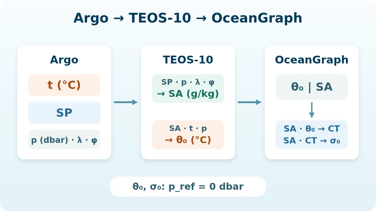
The type of salinity must also be explicit. OceanGraph uses Absolute Salinity (SA), not the Practical Salinity stored as PSAL in the original Argo profile. Potential Temperature and Absolute Salinity Explained covers that conversion and its units.
Pycnocline: A Strong Density Gradient
A pycnocline is a layer where density changes rapidly in the vertical. In a stably stratified water column, density increases downward through it.
This is not safely identified by plotting raw in-situ density against pressure and looking for any increase. In-situ density changes with pressure even for a parcel whose underlying water properties are otherwise comparable. Upper-ocean structure is commonly assessed with potential density referenced to a stated pressure, or with a buoyancy-frequency diagnostic that handles the vertical density gradient consistently.
OceanGraph’s θ-S diagram shows potential density anomaly referenced to 0 dbar (σ₀) as background contours. Those contours help reveal how a temperature-salinity change crosses density space, but the diagram does not itself show the vertical order of the samples. Return to the profile view to locate the change in pressure.
The TEOS-10 standard calculates in-situ density from Absolute Salinity, Conservative Temperature, and sea pressure. Potential density is a separate calculation that also specifies the pressure to which a parcel is referenced; σ₀ uses 0 dbar.
Why the Three Clines May or May Not Align
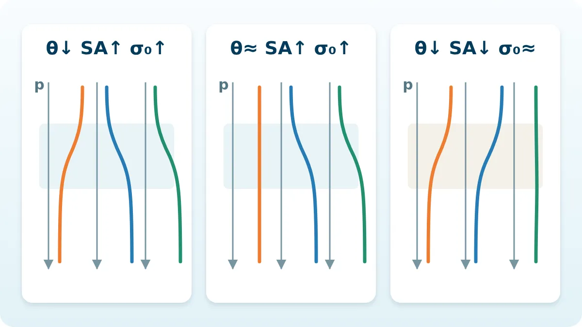
At the same pressure, colder seawater is generally denser than warmer seawater, and saltier seawater is generally denser than fresher seawater. The magnitude of each effect depends on the seawater state, so the result must be calculated rather than inferred from arrows alone.
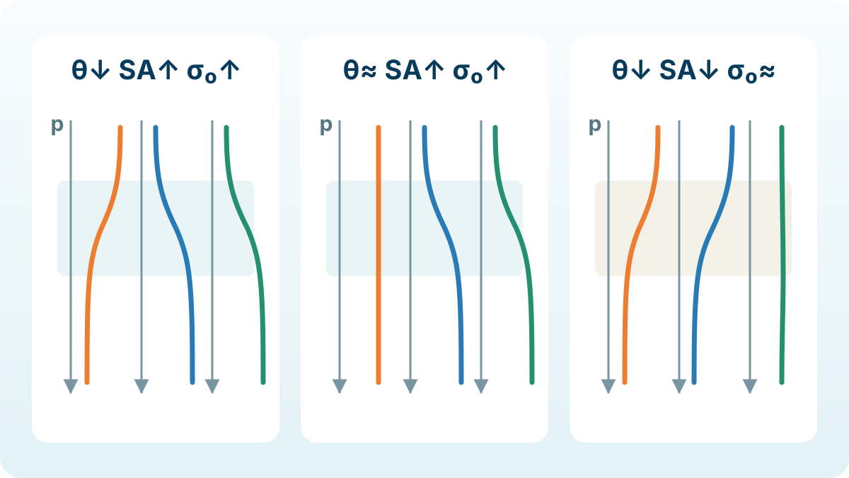
Each variable uses an independent schematic horizontal scale.
Three conceptual patterns are especially useful.
1. Temperature and salinity reinforce each other
Suppose the profile changes downward from warm, relatively fresh water to cold, saltier water. Cooling and increasing salinity both favor denser water below.
In this case:
- The thermocline and halocline may occupy a similar depth range.
- Their density effects reinforce each other.
- A strong pycnocline is likely to occur in the same general interval.
2. Salinity controls the pycnocline
Now suppose temperature changes little while fresh surface water overlies saltier water. There may be no distinct thermocline, but the halocline can create a pronounced pycnocline.
This is one reason a temperature profile alone can miss important upper-ocean stratification. In freshwater-influenced regions, salinity may set the effective barrier between the surface and subsurface ocean.
3. Temperature and salinity partly compensate
Consider warm, salty water above colder, fresher water. Cooling downward tends to increase density; freshening downward tends to decrease it. The two property profiles can each show a sharp cline while the density change is much smaller.
This is called density compensation when the opposing effects substantially offset one another. Depending on the magnitude of the changes, the pycnocline may be weak, shifted relative to the property gradients, or still pronounced.
Observed upper-ocean profiles include cases in which salinity compensates much of a temperature gradient. A peer-reviewed example is discussed by Sérazin and colleagues (2023).
Thermocline, Pycnocline, and Mixed Layer Depth Are Not the Same
These terms answer different questions:
| Term | Meaning |
|---|---|
| Mixed layer | A near-surface region whose properties are relatively uniform |
| Mixed layer depth (MLD) | One estimated value for the lower limit of that region, based on a stated criterion |
| Cline | A finite-thickness region where one variable changes rapidly |
The top of an upper-ocean pycnocline may lie near an MLD estimate, but the two are not definitions of each other. In a threshold-based MLD method such as OceanGraph’s, the algorithm finds a change relative to a shallow reference value. Other MLD methods can locate gradients or fit layer shapes. A cline analysis may identify a gradient maximum or a whole transition range.
They can diverge when:
- Temperature and salinity compensate
- A fresh surface layer creates a shallow density transition above a deeper isothermal layer
- The profile contains several gradient peaks
- Stratification is weak and gradual
- Different MLD criteria or shallow reference depths are used
The fresh-layer case is related to a barrier layer, in which a salinity-controlled density layer limits mixing while nearly uniform temperature extends deeper. For a detailed comparison of threshold choices and barrier-layer logic, see How to Calculate Mixed Layer Depth From a Profile. OceanGraph’s own exploratory MLD definition is documented in Mixed Layer Depth Explained.
How to Identify the Clines in an Argo Profile
Use a paired, definition-first workflow.
1. Check profile quality and vertical coverage
Confirm that temperature, salinity, and pressure are valid over the interval of interest. A gap can make a line segment look like a sharp gradient even though the transition was not resolved. Argo profiles also do not all use identical vertical sampling schemes; the Argo Data FAQ explains relevant sampling and data-use considerations.
OceanGraph displays and exports values after applying its filtering policy, with unavailable cells left missing. Inspect the corresponding Argo NetCDF file to review the source QC arrays and raw-versus-adjusted selection metadata.
2. Compare θ and SA against the same pressure axis
Find the intervals where potential temperature and Absolute Salinity change most rapidly, then compare the direction of change, pressure ranges, and boundary positions.
3. Evaluate the combined density effect
Use the vertical profiles to identify the pressures on either side of a candidate interval, then compare those matched θ-SA points against σ₀ contours. A segment across several contours suggests a larger potential-density change; one running roughly along a contour suggests compensation.
For a quantitative pycnocline depth or strength, export the quality-controlled data and calculate a consistently referenced density or buoyancy-frequency profile. Use the same gradient method, smoothing, and threshold across the profiles being compared.
4. Compare MLD without treating it as the answer
An MLD marker is a useful orientation point. Ask whether it lies near the top of a candidate gradient range and which properties change around it. Recalculate from the profile to identify which temperature, salinity, or density criterion determined the MLD.
5. Repeat across nearby profiles or cycles
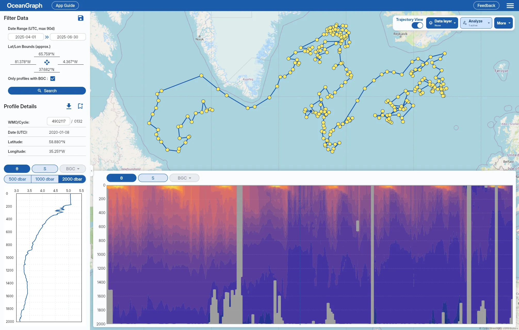
A feature repeated in several coherent profiles is easier to trust than one isolated bend. Keep in mind that an Argo float drifts: differences between cycles combine time evolution and movement through space.
Explore Candidate Clines in OceanGraph
With OceanGraph, you can:
- Compare potential-temperature and Absolute-Salinity gradients on a common pressure axis
- Use θ-S density contours to examine reinforcement or compensation
- Compare the displayed MLD with candidate transition ranges
- Follow changes across a float trajectory and time-series vertical section
Relevant feature documentation includes: