Mixed Layer Depth (MLD) Explained: Calculation and Seasonal Patterns

If you have read a few temperature or salinity profiles, you have probably already noticed it: a shallow layer near the surface where values barely change, followed by a zone where they change quickly. That near-uniform surface layer is the mixed layer, and its depth, the mixed layer depth (MLD), is one of the most widely used indicators in physical oceanography.

MLD is useful because it summarizes, in a single number, how deep wind mixing and surface cooling have stirred the upper ocean. It also sets the stage for other structure you may already be looking at, including the subsurface oxygen maximum and mode water layers.

This guide explains what mixed layer depth means physically, how it is calculated from an Argo profile, why the same water column can have different MLD values depending on the method, and how to read its seasonal cycle using real Argo-based examples in OceanGraph.

If you have not yet read a profile before, start with Ocean Temperature and Salinity Profiles Explained, since MLD builds directly on the surface-layer reading skills covered there.

Why Mixed Layer Depth Matters

The mixed layer is the part of the ocean that exchanges heat, gas, and momentum with the atmosphere most directly. Its depth affects:

• How much of the ocean’s heat content changes for a given amount of surface warming or cooling
• How deep near-surface nutrients, oxygen, and other properties get stirred
• Where the seasonal thermocline sits relative to the surface
• How comparable two profiles really are, since a “surface” value from a 20 m mixed layer and a 150 m mixed layer represent very different volumes of water

Because of this, MLD shows up across oceanography: in air-sea heat budget studies, biogeochemical cycling, mode water formation, and mixed-layer heat content used in seasonal forecasting.

What Mixed Layer Depth Is

Physically, the mixed layer is a near-surface layer that has been homogenized by turbulence, mainly from wind stirring and from convection driven by surface cooling or evaporation. Within that layer, temperature, salinity, and density are close to uniform. Below it, gradients strengthen and the water column becomes more stratified.

MLD is the depth at which that near-uniform layer ends.

How MLD Is Calculated From an Argo Profile

OceanGraph derives MLD from individual Argo profiles as an exploration indicator, using threshold criteria applied to three related quantities.

The three quantities used

• Potential temperature (θ), which removes the effect of compression on temperature so that vertical changes reflect real property differences rather than pressure alone
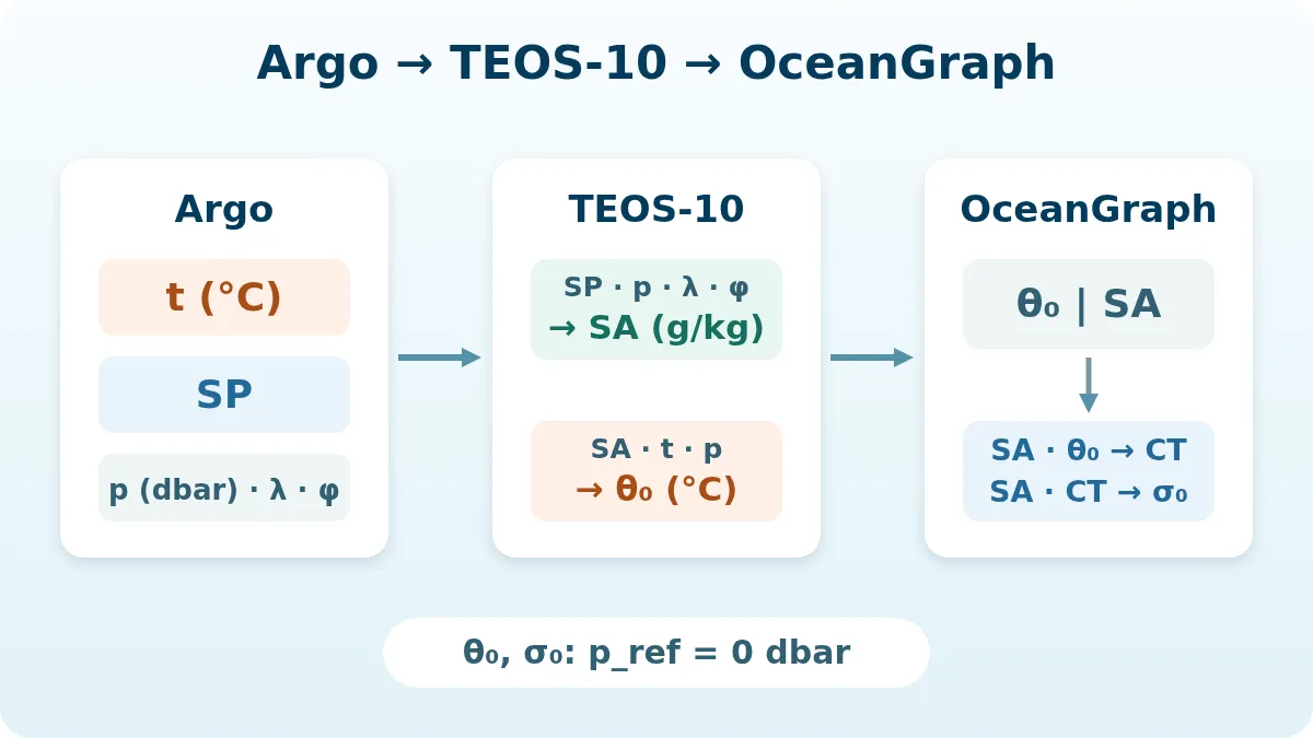
• Absolute salinity (SA), derived from practical salinity, pressure, and position using the TEOS-10 standard
• Potential density anomaly referenced to 0 dbar (σ₀), which combines the temperature and salinity effects into a single density-based view

Because temperature and salinity can partly compensate each other’s effect on density, a method that only checks one of them can miss cases where the water column is well mixed in density but not in temperature, or vice versa. Using all three keeps the definition closer to what “mixed” means physically.

The three threshold criteria

MLD is estimated using three separate threshold tests, each starting from a shallow reference depth (10 dbar):

• Temperature threshold (Δθ): the depth where potential temperature first differs by at least 0.5°C from its value at the reference depth
• Salinity threshold (ΔSA): the depth where absolute salinity first differs by at least 0.05 g/kg from its value at the reference depth
• Density threshold (Δσ₀): the depth where potential density anomaly first differs by at least 0.125 kg/m³ from its value at the reference depth

For each test, OceanGraph finds the first two pressure levels that bracket the threshold and linearly interpolates the pressure where the crossing occurs. It does not simply assign the deeper observation of that pair as the MLD. The three criteria are evaluated independently, and the shallowest interpolated crossing is taken as the MLD. If none of the thresholds is reached anywhere in the profile, MLD is treated as undefined for that observation rather than forced to a value.

If you are choosing a criterion for your own calculation rather than reading OceanGraph’s, How to Calculate Mixed Layer Depth From a Profile works through the four decisions behind numbers like these one at a time.

Data quality requirements

A threshold method is only meaningful if the near-surface part of the profile is sampled well enough to support it. Two coverage checks apply before MLD is calculated:

• Only rows with finite potential temperature (θ) and Absolute Salinity (SA) are used. Their shallowest pressure must be no greater than 30 dbar and their deepest at least 10 dbar. When the first pair lies between 10 and 30 dbar, it supplies the reference values
• The 0–2,000 dbar profile must contain at least three paired rows, including at least two at 50 dbar or shallower

From pressure to depth

Argo measures pressure, not depth directly. OceanGraph records and displays the estimated MLD on the profile’s pressure coordinate in decibars (dbar). Map tooltips and vertical-section data-layer markers use that same value, avoiding a unit mismatch with the section pressure axis. A quantitative conversion from pressure to geometric depth would require latitude-aware processing outside this display contract.

Reading the Seasonal Cycle of MLD

At most mid- and high-latitude locations, MLD follows a clear seasonal pattern driven by the balance between surface heat loss and surface heating.

If your starting question is simply why summer and winter profiles look different, How Deep Do Ocean Seasons Reach? introduces the seasonal water column before the calculation details.

Winter deepening

In winter, surface cooling and stronger winds increase turbulent mixing and reduce the buoyancy of near-surface water. This lets mixing reach deeper, so the mixed layer thickens. In some regions this deep winter mixing is also the mechanism that forms mode water. What Is Mode Water? Formation and Identification follows that connection from the winter mixed layer into the capped subsurface layer.

Summer shallowing

In summer, solar heating warms the surface faster than mixing can redistribute that heat downward. A shallow, strongly stratified layer forms near the surface, and MLD becomes shallow, sometimes only a few tens of meters.

Regional differences

The size of the seasonal MLD cycle is not the same everywhere. Subtropical and mid-latitude regions with strong winter heat loss, such as the western North Pacific south of the Kuroshio Extension, tend to show a large seasonal MLD range. Regions with weaker seasonal forcing, or strong permanent stratification from freshwater input, tend to show a smaller range.

Example: Comparing Two Profiles Across Seasons

Suppose you compare two profiles from a similar location, one from late winter and one from late summer.

A typical pattern would be:

• The late-winter profile shows a deep, nearly uniform temperature and salinity layer extending to well over 100 m, with the density threshold and temperature threshold reaching similar depths
• The late-summer profile shows a shallow uniform layer of only a few tens of meters, followed by a sharp thermocline
• The deeper water below both mixed layers looks relatively similar between the two profiles

This kind of comparison is a practical way to see the seasonal cycle directly in real data, rather than only as a textbook description. It also illustrates why MLD is a useful single number for comparing upper-ocean state across many profiles at once, instead of reading full profile shapes one at a time.

How MLD Connects to Other Structure

MLD is not only useful on its own. In OceanGraph, it also defines the starting point for other derived features:

• The subsurface oxygen maximum (SOM) search begins just below the calculated MLD, so a change in MLD can shift where SOM is found
• Mode water forms through deep winter mixing, so regions and seasons with deep MLD are also where mode water formation is expected

Common Mistakes When Reading MLD

Treating MLD as an exact physical boundary

MLD from a threshold method is an estimate, not a precise physical wall. Real mixed layers can have a gradual transition, and the exact depth depends on the threshold and reference depth chosen.

Comparing MLD values without checking whether MLD was computable

A missing MLD value does not mean zero or an extremely deep mixed layer. It means the profile did not have enough near-surface coverage, or did not cross any threshold. Mixing missing values into an average silently biases the result.

Ignoring the reference depth

Because every threshold is measured relative to a shallow reference depth rather than the true sea surface, profiles with unusual near-surface behavior close to that reference depth deserve a second look before their MLD is trusted at face value.

Reading MLD without season or location context

A 20 m MLD is unremarkable in summer at many latitudes but could be a meaningful signal in winter. Always interpret MLD together with the date and location of the profile.

The Traditional Workflow: Computing MLD From Profiles in Python

A common way to get MLD is to download Argo NetCDF files, convert temperature and salinity to potential temperature and absolute salinity using a toolbox such as GSW, apply a chosen threshold definition, and loop over profiles to build a time series or map.

This is a standard and flexible research workflow, but it has real setup cost:

• You need to choose and implement a specific MLD definition consistently
• You need to handle profiles with insufficient near-surface data
• You need a latitude-aware pressure-to-depth conversion if you want physical depth rather than pressure
• Comparing many profiles across seasons or regions means managing all of this at scale

If your immediate goal is to understand the seasonal MLD pattern in a region, this can be more setup than you need for a first look.

A Better First Step: Explore MLD Visually in OceanGraph

Before writing MLD-calculation code, it often helps to look at the pattern directly:

• Search profiles by region and date range
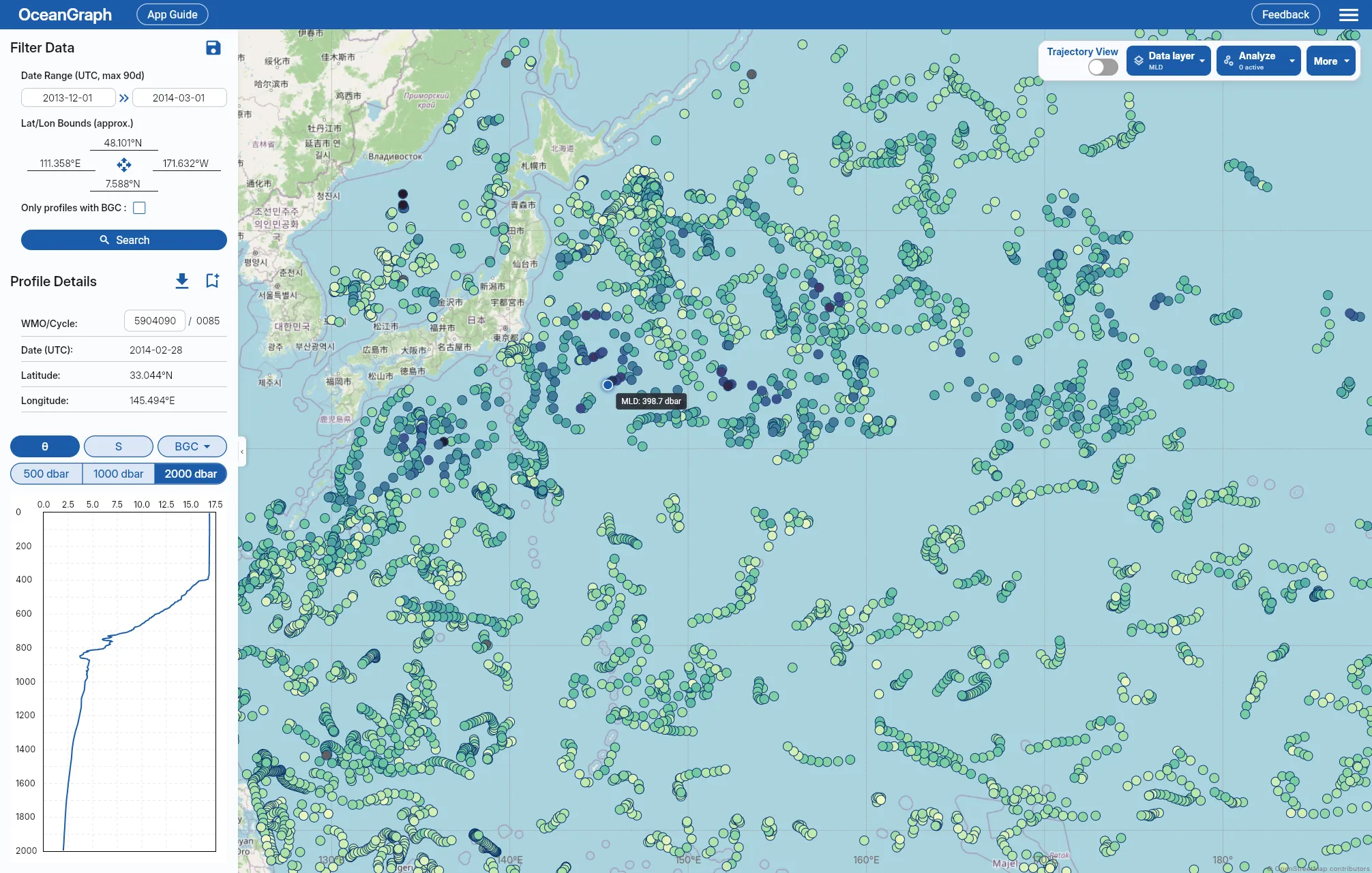
• Select MLD from the Data layer menu to see how MLD varies across many profiles at once
• Compare marker colors between a winter search and a summer search for the same region
• Open individual profiles to confirm what the temperature and salinity structure looks like behind a given MLD value

Useful follow-up pages are:

• Mixed Layer Depth (MLD)
• Analysis Lab: Vertical Profiles (JSON upload)
• Ocean Temperature and Salinity Profiles Explained
• Dissolved Oxygen Profiles in BGC Argo Explained

Explore Mixed Layer Depth in OceanGraph

If you want to move from the definition of MLD to seeing its seasonal cycle in real Argo data, the next step is to compare MLD-colored search results across seasons and regions.

OceanGraph lets you see MLD across many profiles at once, without writing threshold-calculation code yourself.

Frequently Asked Questions

Is there one correct definition of mixed layer depth?

No. MLD depends on the threshold criteria and reference depth chosen. Different reasonable definitions can give somewhat different depths for the same profile. What matters most is applying a consistent definition when comparing profiles.

Why does OceanGraph use temperature, salinity, and density together?

OceanGraph does not blend the three quantities into one combined, density-consistent criterion. It evaluates the temperature, salinity, and density thresholds independently and adopts the shallowest depth where any one of them shows a clear change. This makes MLD a conservative, exploration-oriented indicator: the reported value can end up determined by temperature alone, salinity alone, or density alone, depending on which threshold triggers first at the shallowest depth. Using all three still catches cases that a single-variable method would miss, even though the result is not the same as a strictly density-based definition.

Why is MLD sometimes missing for a profile?

MLD calculation is skipped when the profile does not have enough near-surface coverage, and treated as undefined when none of the threshold criteria are reached anywhere in the profile. Both cases are shown as missing rather than as an approximate value.

How is MLD related to the subsurface oxygen maximum?

OceanGraph evaluates peak shape across the retained source oxygen observations, then accepts only a peak strictly deeper than the calculated MLD. An MLD change can therefore shift which peak is selected, or whether any peak remains eligible. Source oxygen coverage matters independently: for a given peak, observations extending deeper or starting at shallower pressure can preserve or increase its prominence and half-prominence width, making it more likely to pass the shape thresholds. This does not guarantee final selection because the ranking of competing peaks can change too.

Do I need Python to explore MLD patterns?

No. Python is useful for custom MLD definitions or large-scale statistical analysis, but you can compare seasonal and regional MLD patterns visually first, before deciding whether a custom calculation is worth building.

Conclusion

Mixed layer depth condenses the shape of the near-surface water column into a single, comparable number, which is exactly why it is used so widely across oceanography. Reading it well means understanding that it comes from a threshold method, respecting when it is undefined, and always interpreting it together with season and location.

For most learners, the fastest way to build intuition for MLD’s seasonal cycle is to compare profile graphs with the map-level MLD results. That is where OceanGraph helps.