What Is Mode Water? Formation and Identification, With North Pacific Subtropical Mode Water

If you have looked at enough T-S diagrams, you have probably noticed that data points are not spread evenly. In some subtropical regions, a large cluster of points sits at nearly the same temperature and salinity, forming a dense clump instead of a smooth curve. That clustering is not noise. It is the signature of mode water, a distinct type of water mass defined by how common a particular density is across a large regional census of ocean water, not by where it sits geographically.

Mode water matters because it connects several ideas you may have already met separately: deep winter mixed layers, weak subsurface stratification, and the shape of a T-S diagram. Once you can recognize it, several previously separate observations start to fit together.

This guide explains what mode water is, how it forms, how OceanGraph detects it in Argo profiles, and how to identify North Pacific Subtropical Mode Water (NPSTMW) as a concrete example.

Before this article, it helps to already be comfortable with T-S Diagrams in Oceanography Explained (With Examples) and Mixed Layer Depth (MLD) Explained, since mode water sits at the intersection of both topics.

What Mode Water Is

The name “mode water” comes from statistics: if you plot a large volume census of ocean water by temperature and salinity (or density), certain density classes appear far more often than others, forming a mode, a peak in that distribution. Mode water is the water associated with that peak.

Physically, mode water is a thick layer with weak vertical gradients in temperature and salinity, meaning that density changes only slowly with depth through that layer. This is different from a mixed layer at the surface, which is also weakly stratified but sits directly at the surface and is seasonal by nature. Mode water forms in the surface mixed layer during winter, then gets capped by a new seasonal thermocline and persists as a subsurface layer through the rest of the year.

How Mode Water Forms

Mode water formation follows a repeatable seasonal cycle.

Winter: deep mixing creates a thick, uniform layer

In regions with strong wintertime heat loss to the atmosphere, typically along the poleward edge of a subtropical gyre where a strong current such as the Kuroshio Extension recirculates, surface cooling and wind mixing deepen the mixed layer substantially. This is the same deep-winter-MLD process described in Mixed Layer Depth (MLD) Explained. The result is a thick layer of nearly uniform temperature, salinity, and density.

Spring and summer: the layer is capped, not destroyed

As spring solar heating resumes, a new, shallow seasonal mixed layer and thermocline form above the winter layer. The winter layer itself does not disappear. It becomes trapped beneath the new seasonal thermocline, insulated from direct atmospheric forcing, and persists as a subsurface layer with the same weak stratification it had at the end of winter.

Advection: the layer spreads beyond its formation region

Ocean circulation carries this newly capped layer away from where it formed, so mode water is often found well outside its original formation region, embedded as a subsurface layer within profiles that otherwise look unremarkable at the surface.

How Mode Water Is Identified

Because mode water is defined by weak stratification within a density range rather than by a single threshold value, its identification typically combines several criteria.

Density range

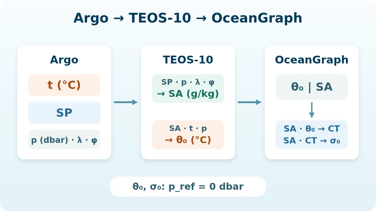
Each mode water type occupies a defined density range that reflects the temperature and salinity conditions present during winter mixing in its formation region. OceanGraph uses potential density anomaly referenced to 0 dbar (σ₀): Absolute Salinity and potential temperature referenced to 0 dbar are converted to Conservative Temperature under TEOS-10 before the configured σ₀ range is applied.

Some literature denotes potential density anomaly as σ_θ. When using published density ranges, check the thermodynamic convention and reference pressure rather than assuming a reported σ_θ value is interchangeable with OceanGraph’s σ₀.

Potential vorticity

Within the target density range, mode water is identified by anomalously low potential vorticity, a quantity that reflects both stratification and rotation. Weak stratification produces low potential vorticity, so a local minimum in potential vorticity within the right density range is a strong indicator of a mode water layer.

Minimum layer thickness

A thin, weakly stratified interval can occur by chance. Requiring a minimum layer thickness helps distinguish a genuine mode water layer from a brief, incidental feature. OceanGraph’s automated detection uses a minimum thickness of 10 m for this purpose.

Geographic bounds

Because each mode water type forms in a specific region, detection is usually restricted to a geographic bounding box for that type. Some operational definitions use a broader box than the strict formation region alone, since it can capture profiles containing advected mode water signals that have moved away from where they formed.

Example: North Pacific Subtropical Mode Water (NPSTMW)

North Pacific Subtropical Mode Water is one of the best-studied mode waters and a useful concrete example.

• Formation region: the recirculation area south of the Kuroshio Extension, in the western North Pacific
• OceanGraph detection range: σ₀ = 25.0–25.6 kg/m³
• Formation mechanism: strong wintertime heat loss from the ocean to the atmosphere over the Kuroshio recirculation gyre drives deep mixed layers, which become NPSTMW once capped by the following spring’s seasonal thermocline

A profile taken well outside the formation region, for example further east in the subtropical gyre, can still show an NPSTMW layer at depth if it sits within the recirculation pathway. That is a direct illustration of advection: the subsurface layer, not the surface conditions at the profile’s location, is what identifies it as NPSTMW.

Other mode water types, such as North Pacific Central Mode Water, South Pacific Subtropical Mode Water, and Atlantic and Indian Ocean equivalents, follow the same general formation logic in their own regions, each with its own density range tied to local winter conditions.

Reading a Mode Water Layer in a Profile

When you inspect a profile that contains mode water, look for:

• A subsurface interval, below the current seasonal mixed layer, where temperature and salinity change only slowly with depth
• That interval’s density falling within the expected range for the mode water type in that basin
• A core depth, which OceanGraph defines as the midpoint of the detected layer after converting its top and bottom pressures to depth (not the depth of minimum potential vorticity), and a layer thickness, the vertical extent over which the weak-stratification criteria are met

Comparing multiple profiles is often more informative than reading one alone, since it shows whether the layer’s thickness and depth are consistent across a region or vary from profile to profile.

Mode Water and the T-S Diagram

Mode water is one of the clearest examples of why a T-S diagram is useful beyond a single profile. If you overlay many profiles from a mode water formation region and its surrounding recirculation pathway, points from the mode water layer cluster tightly together in temperature-salinity space, forming a visibly dense mode rather than spreading along a smooth curve. That clustering is the T-S signature of mode water, and it is the same statistical idea, a mode in a distribution, that gives mode water its name.

Common Beginner Mistakes

Treating any deep, uniform layer as mode water

A uniform layer needs to sit in the right density range and typically needs a minimum thickness before it is treated as mode water. Not every weakly stratified interval qualifies.

Expecting mode water only inside the formation region

Because mode water is advected by circulation, it commonly appears well outside where it formed. A profile far from the named formation region can still contain that region’s mode water.

Confusing mode water with the current season’s mixed layer

Mode water is a subsurface, capped layer from a previous winter’s mixing, not the active surface mixed layer you would identify with a threshold MLD method today.

Assuming a no-detection result means no mode water is physically present

Automatic detection uses fixed geographic, density, potential vorticity, and thickness criteria. A profile can fail one of these operational thresholds while still containing a real but thinner or borderline feature that a manual, research-grade analysis might classify differently.

The Traditional Workflow: Detecting Mode Water in Python

A typical research workflow computes potential density and potential vorticity from Argo temperature and salinity profiles, applies a density-range and potential-vorticity threshold within a chosen geographic box, checks the resulting layer against a minimum thickness, and repeats this across many profiles and seasons to build a time series.

This is a reasonable research pipeline, but it requires implementing density and potential vorticity calculations correctly, choosing consistent thresholds, and managing this across a large number of profiles before you can see whether the pattern you expect is actually present.

A Better First Step: Explore Mode Water Visually in OceanGraph

Before implementing a full detection pipeline, it can help to look at the pattern directly:

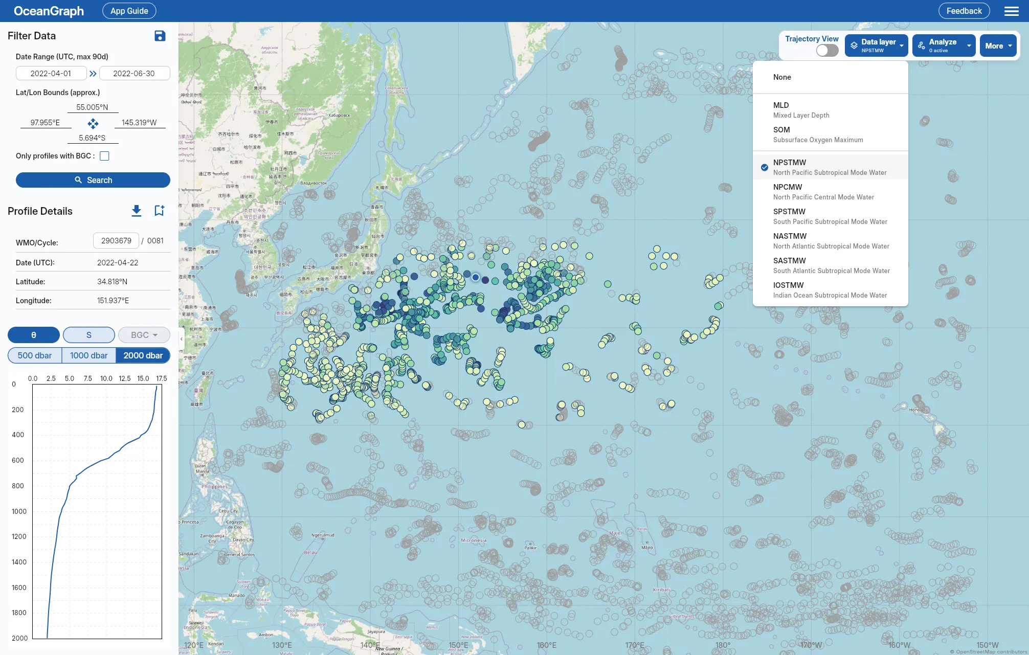
• Search profiles by region and date range
• Select a mode water data layer, such as NPSTMW, from the Data layer menu
• Compare marker colors, which represent detected layer thickness, across profiles in your search results
• Open the Visual Lab Mode Waters view to see seasonal time series of detection counts and thickness for a target region

Useful follow-up pages are:

• Mode Water Data Layer
• Mode Waters (Visual Lab)
• T-S Diagrams in Oceanography Explained (With Examples)
• Mixed Layer Depth (MLD) Explained

Explore Mode Water in OceanGraph

If you want to move from the definition of mode water to seeing it in real Argo profiles, the next step is to compare mode-water-colored search results across a formation region and its surrounding recirculation area.

OceanGraph lets you see mode water detections and their thickness across many profiles at once, without implementing density and potential vorticity calculations yourself.

Frequently Asked Questions

Why is it called “mode water” instead of a water mass name based on location?

The name comes from statistics: it describes water associated with a pronounced mode, or peak, in a volumetric temperature-salinity census, reflecting how common that particular density is compared to surrounding water. Location-based descriptions, such as North Pacific Subtropical, are added to identify which mode water type and formation region is meant.

Is mode water the same as the current mixed layer?

No. Mode water is a subsurface layer, capped by a more recent seasonal thermocline, that originated as a mixed layer in a previous winter. The active surface mixed layer today is a separate, shallower feature identified with a threshold MLD method.

Can mode water be found far from its formation region?

Yes. Ocean circulation advects mode water away from where it formed, so it is commonly detected as a subsurface layer in profiles well outside the strict formation area.

Why does mode water detection use potential vorticity instead of density alone?

Density range alone can include water that is still fairly stratified. Low potential vorticity specifically flags weak stratification within that density range, which is the defining physical property of mode water.

Do I need Python to identify mode water in Argo profiles?

No. Python is useful for custom detection criteria or large-scale statistical analysis, but you can explore where mode water is detected, and how thick it is, visually first.

Conclusion

Mode water connects deep winter mixing, weak subsurface stratification, and T-S diagram clustering into a single, recognizable feature. Once you understand that it forms through deep mixed layers, gets capped by the next season’s thermocline, and is then carried by circulation, individual profiles that seemed unremarkable on their own start to make more sense as part of a larger seasonal and regional pattern.

For most learners, the fastest way to build that intuition is to compare real detections interactively. That is where OceanGraph helps.