On this page
An ocean front is a zone where water properties change rapidly in the horizontal direction compared with the surrounding ocean. Temperature, salinity, density, or other properties may form the gradient.
Maps often draw a front as a line, but a front has width, depth, and structure; it can strengthen, weaken, meander, split, and move. It may separate recognizable water masses, or it may separate regions with different vertical stratification without either side being perfectly uniform.
To explore the subsurface on each side with Argo, compare profiles from multiple locations at common pressures, preferably observed close in time.
What Defines an Ocean Front?
The defining feature is a large horizontal gradient over a relatively narrow zone. For example, if potential temperature at 100 dbar changes much more rapidly across a small geographic interval than it does in the surrounding region, that pattern may indicate a temperature front.
The same logic applies to salinity and density. A hydrographic front may be:
- Temperature-dominated, with a strong horizontal thermal contrast
- Salinity-dominated, with fresher and saltier water meeting
- Density-compensated, where temperature and salinity contrasts oppose each other so the density contrast is weaker
- Density-reinforced, where temperature and salinity both strengthen the density contrast
A global analysis by Belkin, Cornillon, and Sherman (2009) treats major ocean fronts as persistent large-scale gradient features while also documenting their complex, regional structure. “Persistent” does not mean motionless: the instantaneous position can meander around a broader climatological zone.
For the larger vertical setting in which fronts occur, start with How Does the Ocean Change With Depth?.
A Front Is Horizontal; a Cline Is Vertical
This is the most important distinction.
- A thermocline is a strong temperature change down one profile.
- A halocline is a strong salinity change down one profile.
- A pycnocline is a strong density change down one profile.
- A front is a strong property change between horizontal locations.
A profile can contain a sharp thermocline without being near a front. Conversely, two sides of a front may each have smooth vertical profiles but differ greatly from one another at the same pressure.
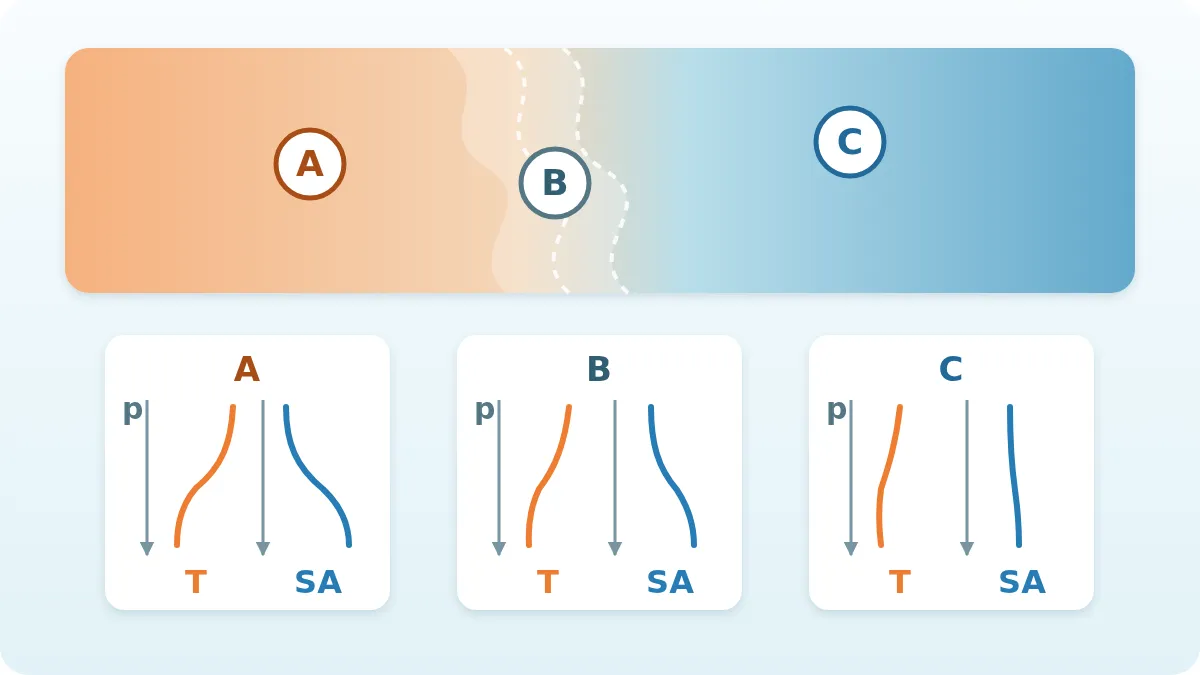
When comparing stations A, B, and C across a suspected front, ask two separate questions:
- How does each profile change vertically?
- How do the profiles differ horizontally at the same pressure?
Thermocline, Halocline, and Pycnocline: What Is the Difference? explains the vertical structures in detail.
A Front Is a Zone, Not a Fixed Boundary Line
Drawing a line is useful for maps and communication, but several choices are hidden in that line:
- Which variable defines the front?
- At what pressure or depth?
- What gradient threshold or contour is used?
- Over what time interval were observations combined?
- Is the line an instantaneous estimate, an average position, or a broad frontal zone?
Different choices can locate different aspects of the same physical system. A surface temperature front can lie away from a subsurface salinity or density front, and the contrast can fade or shift with depth.
The Japan Meteorological Agency’s description of the Polar Front in the Japan Sea provides a useful regional example: temperature and salinity sections show a strong transition near the surface and upper ocean, while the deeper structure does not preserve an identical boundary. The lesson is general even though the example is regional—always ask how far downward the contrast extends.
What Changes Across a Front in Vertical Profiles?
There is no universal “front profile,” but several comparisons are informative.
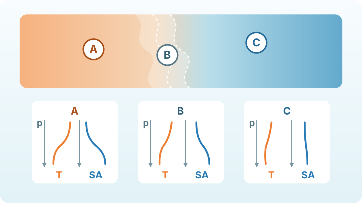
Temperature and salinity use separate schematic scales; real fronts may be dominated by either property, density, or a combination.
Values at common pressure levels
Start with pressures sampled on both sides. Compare θ and SA at 10, 100, 300, or another scientifically relevant level only when all selected profiles have valid nearby observations or have been put on a justified common grid.
A coherent step or steep geographic trend across several adjacent profiles is more persuasive than one unusual pair.
Mixed-layer and cline structure
The two sides may differ in:
- Mixed layer depth
- Thermocline or halocline depth and thickness
- The direction and strength of salinity gradients
- Subsurface temperature or salinity maxima and minima
- The pressure below which the profiles converge
These shape differences can reveal a subsurface front even when surface values look similar. They can also show that an apparent surface boundary is shallow and does not separate the deeper water column.
Vertical reach
Compare the contrast through the whole shared pressure range. A difference confined to the top few tens of decibars describes a different structure from one that persists through hundreds of decibars.
Use a θ-S Diagram to Check Water-Property Contrast
A θ-S diagram removes pressure from the main axes and shows the combinations of potential temperature and Absolute Salinity in each profile. Across a candidate front, it can help you ask:
- Do profiles on the two sides occupy distinct parts of θ-S space?
- Is only the upper part of each curve different, or is the whole curve displaced?
- Do transition-zone profiles have intermediate properties?
- At a pressure matched between the two sides, does the segment joining their θ-SA points cross σ₀ contours or run roughly along one?
Profiles that occupy distinct θ-S ranges support the interpretation that the selected waters differ in their property structure. An intermediate curve may reflect mixing or sampling a transition zone.
To assess frontal density compensation, match θ and SA at the same pressure in the profile data, calculate density consistently for each location, compare the resulting values, and use the θ-S view as supporting context. T-S Diagrams in Oceanography Explained covers the general reading method.
A Temperature Front Is Not Automatically a Density Front
Suppose one side is warm and salty while the other is cold and fresh. The temperature contrast and salinity contrast affect density in opposite directions. A strong temperature front can therefore have a smaller potential-density contrast than expected.
The reverse is also possible: cold, salty water next to warm, fresh water makes both properties reinforce the horizontal density gradient.
This matters because density gradients are connected to pressure gradients and circulation, while a temperature image alone shows only the thermal component. Before calling a hydrographic feature a density front, calculate density for each same-pressure temperature-salinity pair with a consistent equation of state, then compare the resulting densities across locations. Spiro Jaeger and Mahadevan (2018) provide an observational analysis of temperature-salinity compensation at ocean fronts.
An Ocean Front Is Not the Same as a Current or a Surface Slick
Fronts and currents are often related, but the terms are not synonyms. A current describes water motion. A front describes a property gradient. A strong current can follow or help maintain a front, yet temperature and salinity profiles contain no direct velocity measurement.
Likewise, a visible surface line, foam streak, color change, or convergence slick can occur near a water-mass boundary, but appearance alone does not establish the full hydrographic front. The surface sign may be shallow, transient, or generated within broadly similar water.
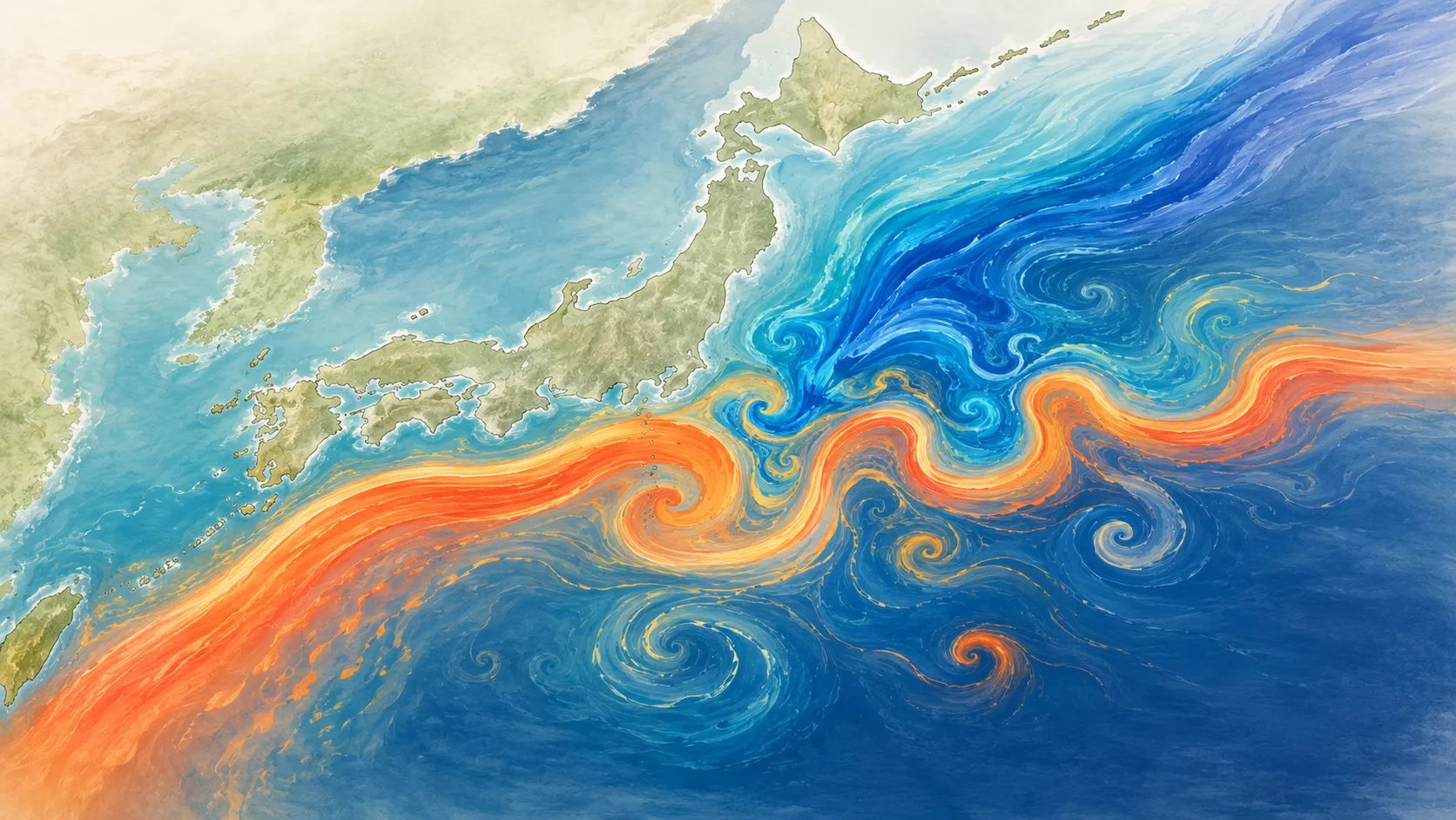
If your main question is why currents form and what a profile can reveal about them, read What Causes Ocean Currents?. For a concrete regional comparison, Kuroshio and Oyashio Below the Surface shows how water properties differ around two major western North Pacific current systems.
A Careful OceanGraph Workflow
Map search and marker context are available without an account. The selected profile graph, θ-S diagram, downloads, and Analysis Lab comparison require signing in.
1. Define a focused region and short time window
Search across the suspected frontal zone, not only along one side. Keep the period as short as practical while retaining enough profiles. Combining distant seasons can turn temporal change into an apparent horizontal gradient.
2. Inspect profiles across a geographic transect
Identify several markers extending from one side through the transition to the other. OceanGraph keeps one map marker selected at a time, so click them in geographic order and check each date, latitude, longitude, WMO ID, and cycle before comparing values.
3. Compare vertical profiles at shared pressures
Inspect potential temperature and Absolute Salinity together. Note the values at common pressures, profile shapes, mixed layer depths, cline positions, and the pressure to which differences persist. For a side-by-side overlay, download the relevant profile JSON files and upload them to the desktop Analysis Lab: Vertical Profiles viewer.
4. Generate θ-S for the focused result set
With Trajectory off, θ-S uses the entire current search result, not a hand-picked subset; keep the result at 500 profiles or fewer. Select markers one at a time to highlight their curves and look for coherent separation between sides. Use the contours as density context, but test reinforcement or compensation with same-pressure pairs outside the curve-only display.
5. Check repetition, missing values, and source quality
Repeat the comparison with nearby profiles or a neighboring time window. A pattern that depends on one unusual observation is weak evidence. OceanGraph shows values after its published filtering policy and preserves gaps as missing values, but it does not expose the source QC arrays in the profile view or downloaded JSON. To review the original QC flags, separately download the corresponding NetCDF file from an Argo GDAC and inspect the arrays in that file.
6. Use time sections and clustering as supporting views
A float’s time-series vertical section can show when its observed structure changed. But the float also moved, so the section combines space and time. Its trajectory is not a surface-current streamline because a core Argo float spends most of its cycle drifting at depth.
Clustering can highlight groups with different profile structure, but a cluster-color boundary is only a hypothesis about a front. Search limits, date, shared depth coverage, standardization, and geographic features all influence the result. Ocean Profile Clustering Explained describes those dependencies.
The relevant feature guides are:
- Search and Bookmark
- θ-S Diagram
- Analysis Lab: Vertical Profiles
- Trajectory and Time-Series Vertical Section
- Clustering
- Data Filtering Policy
How Strong Is the Evidence?
It helps to treat front identification as an evidence ladder.
A candidate front
Several nearby profiles show an organized horizontal temperature or salinity contrast at common pressures over a focused period.
A stronger hydrographic interpretation
The contrast repeats across neighboring observations, has coherent vertical structure, remains credible after reviewing missingness and the source Argo QC information, and is consistent in the map, profile, and θ-S views.
A quantitative front analysis
The study defines a horizontal gradient metric, pressure level or layer, time window, interpolation method, uncertainty, and front-position rule. It may add satellite sea-surface temperature, sea-surface height, ship or glider sections, and velocity observations to resolve scales that sparse Argo sampling cannot.