
On this page
A water mass is a body of seawater with a shared formation history and a recognizable range of properties. Temperature and salinity are central to that description because surface heating, cooling, evaporation, precipitation, ice processes, and mixing leave a combined signature that can persist after the water enters the ocean interior.
What Oceanographers Mean by a Water Mass
A practical definition has two parts:
- The water shares a formation history, associated with a source region or set of processes.
- It occupies a range of properties that can be traced beyond that formation region.
The range may include potential temperature, salinity, potential density referenced to a stated pressure, dissolved oxygen, nutrients, or other tracers. Temperature and salinity are usually the starting point because they carry information about formation and later modification. Quantitative density comparisons additionally require an equation of state and either the in-situ pressure or a stated reference pressure.
Several related terms describe different things:
| Term | Meaning | Example question |
|---|---|---|
| Water parcel | A small conceptual amount of water followed through space and time | How did this parcel change? |
| Water type | An idealized temperature-salinity combination, sometimes represented by a very narrow range in practice | What temperature-salinity combination does this point represent? |
| Water layer | Water occupying a depth interval at one place and time | Where is the low-salinity layer? |
| Water mass | A body of water connected by formation history and a property range | Does this recurring signature fit a known source and pathway? |
A water type can be drawn as a point in temperature-salinity space. A water mass can occupy a line, band, or region in that space because its properties vary and because it mixes with other water. The distinction is described in the University of Hawaiʻi’s water-mass formation notes and in Robert Stewart’s institutional textbook, Introduction to Physical Oceanography.
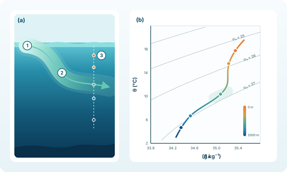
In panel (a), 1 marks the near-surface formation region, 2 the layer’s spreading and modification, and 3 one vertical sampling profile. Its five sample points run from warm colors near the surface to blue at depth, with the water mass surrounding the third point. Panel (b) uses the same five colors and places a softly bounded candidate property range around the matching third point.
How a Water Mass Acquires Its Signature
Many water masses begin with processes acting at or near the sea surface, where the ocean exchanges heat and freshwater with the atmosphere and cryosphere. Cooling lowers temperature. Evaporation removes freshwater and raises salinity. Rain, river input, and melting ice tend to freshen the surface. Sea-ice formation rejects much of the salt into the remaining water. Wind and convection then mix those effects through a surface layer.
These processes do not produce a universal warm-salty or cold-fresh relationship. Their balance depends on region and season. Cooling and brine rejection at high latitudes can create dense water that sinks, while winter mixing and subduction in a subtropical region can move a different property range beneath the seasonal surface layer. NOAA’s thermohaline circulation explanation gives a clear high-latitude example, and Scripps Institution of Oceanography’s upper-ocean water-mass notes describe how surface-layer properties enter the ocean interior.
Formation, Spreading, and Modification Are Different Stages
It helps to separate three questions that are often compressed into one name.
Where and how did the water form?
This concerns the processes that established its properties. Surface heat and freshwater fluxes, sea-ice processes, winter mixing, convection, and interaction with neighboring waters can all matter.
Where did it spread?
Advection can carry the water far from its source. Finding a signature at one location therefore does not mean that it formed there. A current is the motion; a water mass is the water characterized by its history and properties.
How was it modified?
Water masses mix with surrounding water as they move. Their temperature-salinity range can broaden or shift, and oxygen or nutrient signatures can evolve through biological and chemical processes. Boundaries between named masses are therefore often transitional rather than sharp.
What a T-S Diagram Adds
A vertical profile shows where temperature and salinity occur with pressure or depth. A T-S diagram removes depth from its main axes and places each valid temperature-salinity pair in property space. Repeated curves, bends, extrema, and compact bands can then make related water easier to compare.
If you are still learning the axes and basic curve shapes, begin with T-S Diagrams in Oceanography Explained. The present article addresses the next question: when does a pattern support a water-mass interpretation?
Useful signs include:
- A similar temperature-salinity branch recurring across neighboring profiles
- A subsurface salinity maximum or minimum at a consistent density or depth range
- A compact property range that persists while the surface part of the profiles changes
- Intermediate values lying between plausible source-water endpoints
A branch can combine several source waters, seasonal sampling can alter the apparent range, and different processes can produce similar temperature-salinity combinations.
A σ₀ contour on a T-S diagram connects temperature-salinity pairs with the same potential-density anomaly referenced to 0 dbar. It shows that the water parcels would have the same density if moved adiabatically to 0 dbar; it does not imply that they occupy the same depth or layer, or that they followed the same pathway. Pressure increases with depth and compresses seawater, but the amount of compression depends on temperature and salinity. Two water parcels with the same density when referenced to 0 dbar can therefore have different densities at the same pressure in the deep ocean. Use σ₀ contours to compare density, and assess water-mass origins and pathways using location, depth, and other tracers. The theoretical basis for this distinction is explained in the primary paper Neutral Surfaces.
End-members and mixing paths
An end-member is a representative set of source-water properties used to interpret mixtures. Here, a conservative mixing variable is one whose value, at a common pressure and without external input of heat or matter, follows the mass contributions from the sources. If two fixed end-members mix and temperature and salinity can be treated as conservative variables during mixing, the resulting water falls along the mixing line between them.
Real-ocean evidence is less tidy. The end-members themselves can vary, more than two waters may contribute, and samples collected at different places or times may be placed on the same plot. A straight-looking segment is therefore consistent with simple mixing, not proof that only two fixed sources produced it.
The TEOS-10 Manual adds a thermodynamic caveat. Absolute Salinity is conserved under turbulent mixing, although biogeochemical changes in seawater composition can modify it. Potential temperature is preserved when a parcel changes pressure isentropically and without a salinity change, but it is not exactly conservative during mixing. Conservative Temperature is much closer to a conservative heat variable. Density and potential density are derived, non-conservative quantities that respond nonlinearly to mixing.
For quantitative work under TEOS-10, use variables and equations that match the calculation. TEOS-10 recommends Absolute Salinity and Conservative Temperature for water-mass analysis and potential-density calculations, as summarized in Getting Started with TEOS-10. Potential Temperature and Absolute Salinity Explained covers the variables used by OceanGraph and how they differ from an SA-CT diagram.
From a Candidate Signature to a Named Water Mass
Treat identification as an evidence ladder rather than a one-step visual match.
1. Find a coherent property pattern
Look for a recurring range, extremum, or branch across more than one profile. One unusual curve may reflect a sensor issue, missing values, a transient feature, or an unrepresentative time and place.
2. Restore depth, location, and time
Determine where the candidate range occurs in each profile and whether the geographic and seasonal setting is plausible. Read depths from the vertical profiles or from depth labels or colors added to the T-S diagram.
3. Compare with an expected formation region and spreading path
Identification with a named water mass should be grounded in regional literature describing where the water forms, the density or depth range it occupies, and how it spreads.
4. Add complementary evidence
Dissolved oxygen, nutrients, transient tracers such as CFCs, potential vorticity, and velocity or circulation context may support or challenge the interpretation. These quantities are not all independent of temperature and salinity—potential vorticity, for example, depends partly on density stratification—but each can test a different aspect of the water’s age, modification, layer structure, or route.
5. Check the identification criteria
A reproducible analysis identifies the variables, thresholds or property ranges, reference pressure, region, time period, and data-quality rules. If those checks have not been completed, “candidate signature” or “water consistent with” is more accurate than a definitive name.
Water Mass Is Not a Synonym for Layer, Front, or Mode Water
A layer answers where water lies vertically at a particular place. The same water mass can appear at different depths as density surfaces rise and fall, and one depth interval can contain mixtures of several masses.
An ocean front is a zone of enhanced horizontal property gradients. A front may separate water masses, but the gradient itself is not a water mass. What Is an Ocean Front? explains how multiple profiles are needed to identify a candidate boundary.
Mode water is a particular class of water mass associated with a large volume in a narrow property range and commonly observed as a thick, weak-gradient layer. Formal detection can require density, layer thickness, potential vorticity, and geographic criteria; it is not simply any tight cluster on a T-S diagram. See What Is Mode Water? for the North Pacific subtropical example.
Exploring Water-Mass Evidence in OceanGraph
OceanGraph supports the exploratory stage: finding profiles, comparing their vertical structure, and checking whether a θ-S pattern recurs. OceanGraph has a separate map feature that displays mode-water detections using predefined criteria for each mode-water type.
- Choose a focused region and period. A compact search makes geographic and seasonal interpretation clearer. With Trajectory off, θ-S uses all current search results; keep the result to 500 profiles or fewer.
- Read the vertical profiles first. Note where potential temperature and Absolute Salinity extrema or low-gradient layers occur, together with the profile date, position, WMO ID, and cycle.
- Generate θ-S and highlight profiles. Signed-in users can open Analyze and select Generate θ-S. Selecting a map marker highlights that profile’s curve against the result set. With Trajectory on, the input is every loaded cycle for the selected float, again up to 500.
- Check the candidate feature’s depth and distribution. Determine whether it occurs at a consistent pressure range and repeats in nearby profiles or cycles. Use background σ₀ contours for density and the vertical profile for the pressure range.
- Verify before formal analysis. OceanGraph plots quality-filtered potential temperature against Absolute Salinity. It omits a selected curve with fewer than two finite pairs, and profile data downloaded from OceanGraph do not include the source QC flags. Review the original Argo NetCDF and regional literature before adopting a formal identification.
OceanGraph converts potential temperature to Conservative Temperature internally when calculating the σ₀ background contours; the plotted vertical axis remains potential temperature. The exact controls and display contract are documented in the θ-S Diagram App Guide, while the Data Filtering Policy explains which source values reach the display.