What Is bbp700? Reading Particle Backscattering in BGC Argo

BGC Argo floats use light to detect particles suspended in seawater. The resulting particulate backscattering coefficient at 700 nm, or bbp700, describes how strongly particles scatter that light backward. Its vertical profile helps locate particle-rich layers, but the value is not a particle count or a direct measurement of living plankton biomass.

The BGC Argo sensor overview places backscattering alongside oxygen, chlorophyll, nitrate, pH, and light.

What the Sensor Measures

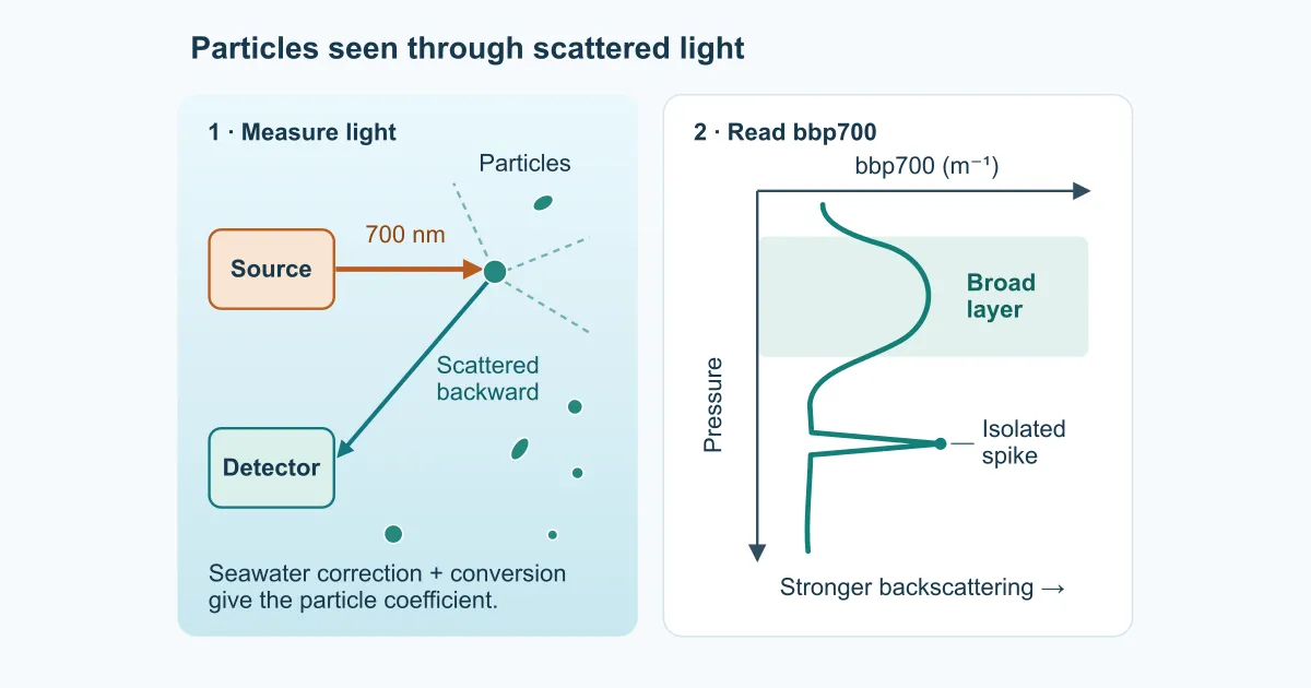
A backscattering sensor emits light and detects some of the light scattered through a particular backward angle. Processing removes the estimated contribution from seawater itself, then converts the particle signal at that angle to a coefficient representing scattering into the backward hemisphere. Dall’Olmo and colleagues (2023) describe this conversion.

In bbp700, 700 refers to the light’s wavelength, 700 nanometers. The coefficient has units of m⁻¹, describing backscattering per unit path length. A larger value means stronger particulate backscattering at that wavelength.

Particles include living microorganisms, organic debris, and inorganic material. Their sizes and composition affect how they scatter light, so twice the bbp700 does not necessarily mean twice as many cells or twice as much particle mass. Koestner and colleagues (2022) examine why particle properties complicate optical estimates of carbon.

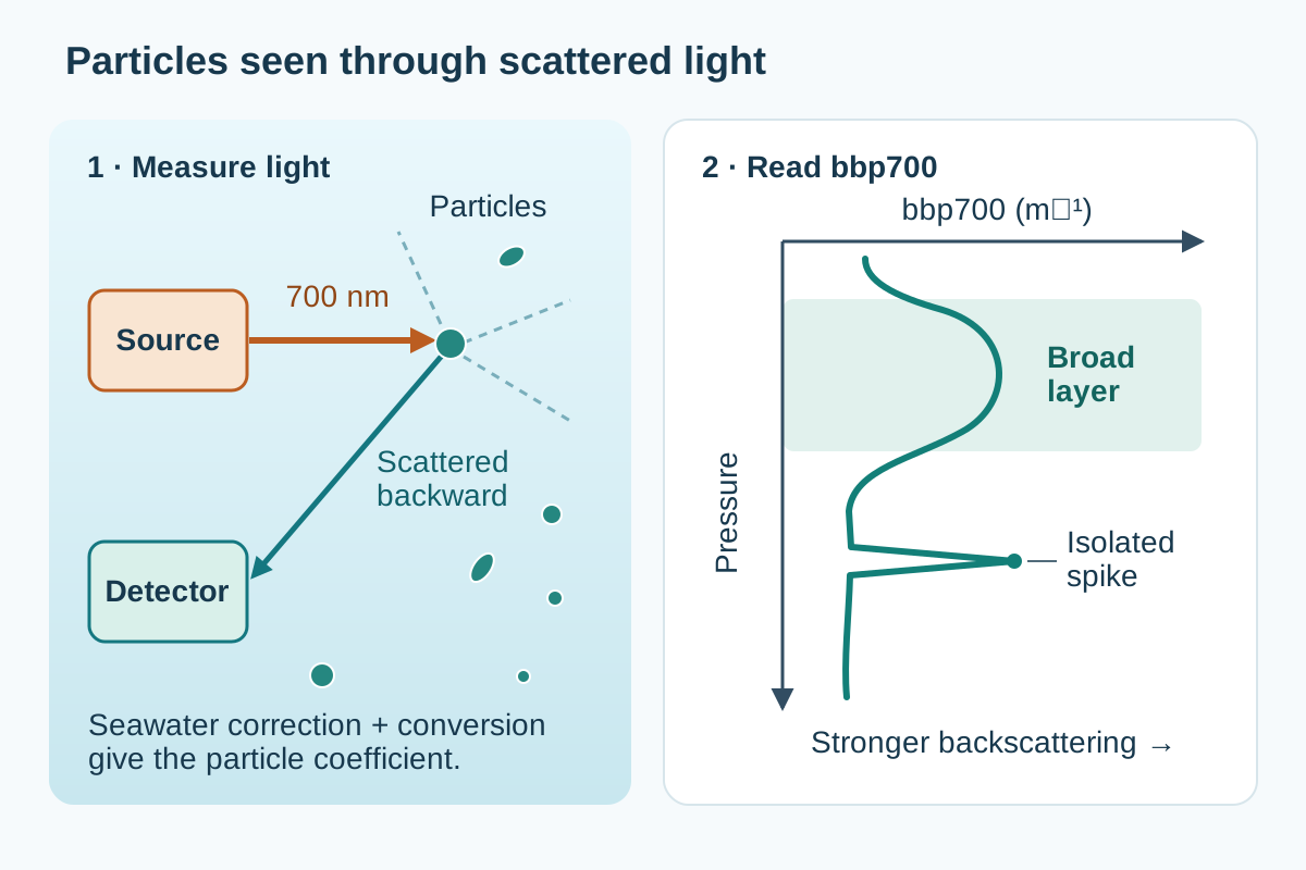
The detector samples light at a particular angle. The profile on the right shows the derived bbp700: pressure increases downward, while stronger backscattering appears farther to the right.

Broad Layers and Sharp Spikes Need Different Interpretations

A sustained increase over several neighboring measurements outlines a layer with stronger backscattering. Check its upper and lower boundaries, how it aligns with temperature and salinity changes, and whether a similar feature appears in nearby cycles. Those comparisons help distinguish a persistent layer from an isolated encounter with a particle. The float moves between cycles, so a changing profile can also reflect movement into different water.

A narrow spike is more ambiguous. Large aggregates can produce real, brief peaks when they pass through the sensor’s small sampling volume. Animals can also produce strong optical signals: Haëntjens and colleagues (2020) linked spike layers to mesopelagic organisms and suggested that attraction to float sensor lights contributed to the signals. Instrument or processing problems are other possibilities. Neither automatically deleting every spike nor interpreting every spike as sinking organic matter is justified.

The BGC Argo suspended-particle overview explains how repeated optical profiles support studies of particle transport. For an initial reading, compare the background profile and the localized peaks separately.

Compare bbp700 With Chlorophyll

Backscattering responds to particles, whereas chlorophyll fluorescence responds to a photosynthetic pigment. Comparing them at the same pressures adds information that either profile alone lacks:

• Both increase in the same layer: a phytoplankton biomass increase is plausible.
• Chlorophyll increases without a comparable bbp700 increase: cells may contain more pigment relative to carbon as they acclimate to dim light.
• bbp700 increases without a chlorophyll peak: nonalgal particles may contribute, but particle properties, chlorophyll physiology, and data quality also need examination.

These comparisons require overlapping valid measurements. For the distinction between pigment and biomass maxima, including the effects of daytime fluorescence suppression, see Deep Chlorophyll Maxima Explained.

From Backscattering to Carbon: An Extra Inference

Researchers use empirical relationships to estimate particulate organic carbon (POC) from backscattering. Such relationships are fitted to optical observations and measurements of carbon in water samples; they are not unit conversions. Their applicability depends on the particle population, wavelength, and conditions represented in the calibration dataset. The Koestner et al. study shows why including chlorophyll can help account for differences among particle assemblages.

POC concentration describes carbon present per unit volume. A sinking carbon flux describes carbon crossing a unit area per unit time. Moving from one to the other needs information about transport, such as sinking speed, or an explicit model using repeated observations. Estapa and colleagues (2017) discuss float-based approaches and the effects of sampling and horizontal transport.

Particles and oxygen offer complementary information about the biological carbon cycle. Where Is Oxygen Found in the Ocean? explains how respiration and ventilation shape oxygen below the sunlit layer; neither oxygen nor particles should be read without the circulation context.

Check Quality Before Quantitative Use

Inspect the original Argo backscattering quality flags and processing status before calculating particle or carbon statistics. Real-time screening can flag suspicious profile shapes without establishing their exact cause. In the backscattering quality-control study, flag 3 means probably bad data requiring expert examination.

This matters when exploring OceanGraph. Its publishing policy masks selected-source BGC flags 4 and 9, so a plotted value does not necessarily have flag 1 or 2. The Data Filtering Policy explains source selection and masking. Missing values remain missing, rather than becoming zero particle concentration. For the broader meaning of data modes, adjusted variables, and flags, read Argo Data Quality Control.

Read a Particle Profile in OceanGraph

1. Search a region and date range, enabling Only profiles with BGC. This includes profiles with any supported BGC variable, so check that the selected profile actually contains backscattering.
2. Select the BBP chart. OceanGraph labels the plotted variable BBP (m⁻¹) and uses the bbp700 field.
3. Follow the curve over its observed pressure range. Separate sustained layers from isolated peaks and inspect where measurements are missing.
4. Compare chlorophyll, temperature, and salinity over the same pressure range, then inspect neighboring cycles and the float’s positions.

The Search and Bookmark guide covers profile discovery and downloads. After signing in on a desktop or laptop computer, you can use Analysis Lab’s Vertical Profiles viewer to compare the depth and persistence of particle layers across several downloaded JSON profiles.