On this page
An ocean eddy can deepen or lift the layers beneath the sea surface, so two nearby profiles may have different temperatures at the same depth. Warm-core eddies often contain a thicker warm upper layer; cold-core eddies often bring the colder layers closer to the surface. Reading that structure requires salinity and a suitable comparison profile, as well as temperature.
The terms describe a contrast with surrounding water, not a fixed temperature threshold.
What Is a Mesoscale Ocean Eddy?
An eddy is a circulating feature in the flow. Ocean currents can meander and shed eddies, as NOAA’s introduction to eddies illustrates. Here the focus is the large open-ocean features called mesoscale eddies, rather than small tidal whirlpools.
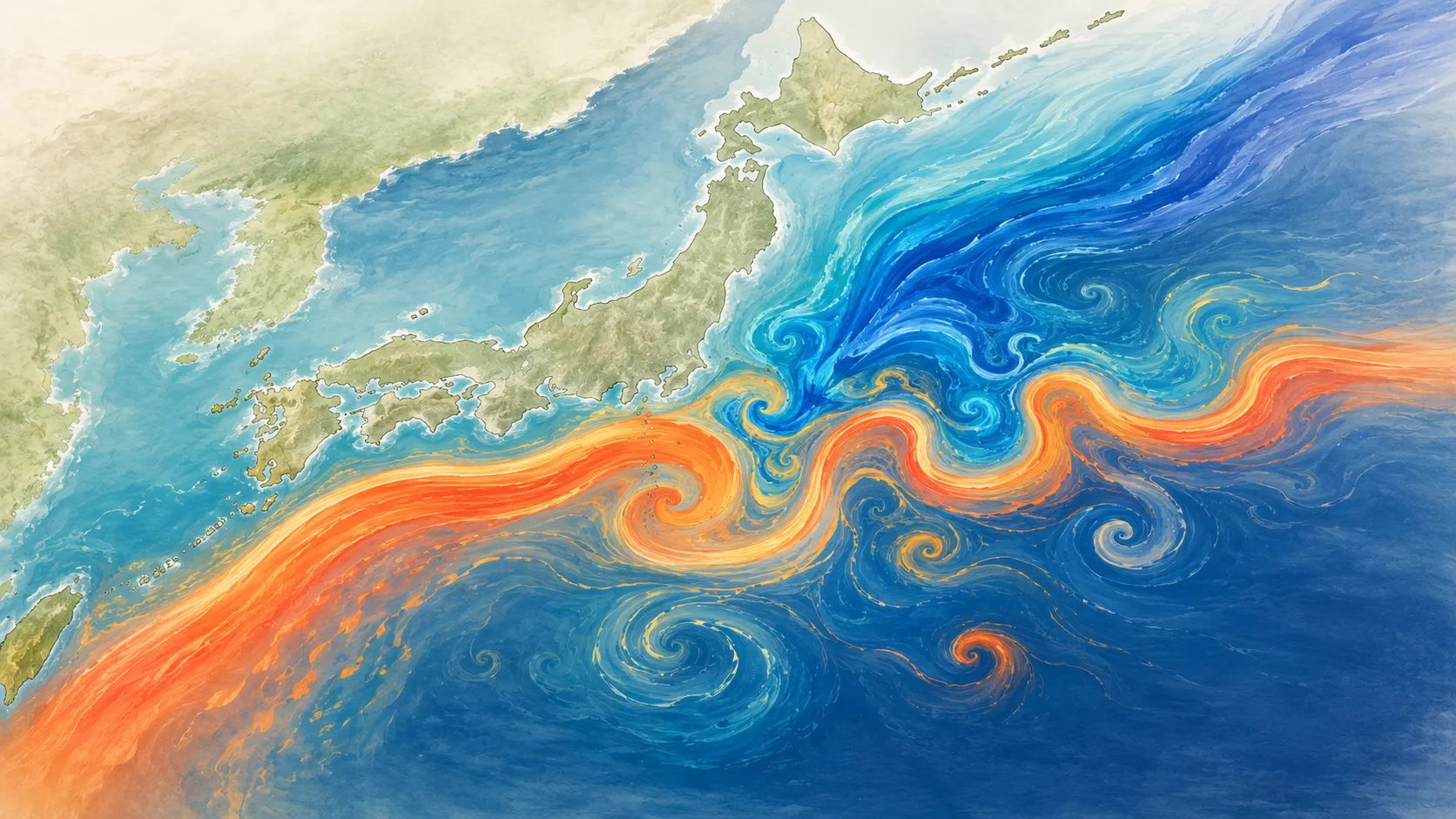
Features around 100 km across are widespread, and the Kuroshio Extension east of Japan is an especially active region. Eddies there can carry warm water away from the main current and alter the surrounding ocean structure. JAMSTEC’s explanation of eddy activity describes that setting. For its broader water-property contrast, see Kuroshio and Oyashio Below the Surface.
Rotation and thermal structure describe different aspects of an eddy:
| Rotation type | Northern Hemisphere | Southern Hemisphere |
|---|---|---|
| Cyclonic | Counterclockwise | Clockwise |
| Anticyclonic | Clockwise | Counterclockwise |
For many eddies with a clear sea-surface-height signal, anticyclonic rotation accompanies elevated sea level and a warm core, while cyclonic rotation accompanies lower sea level and a cold core. AVISO’s overview of eddies tracked by altimetry explains this common association.
The Layers Bend Beneath the Eddy
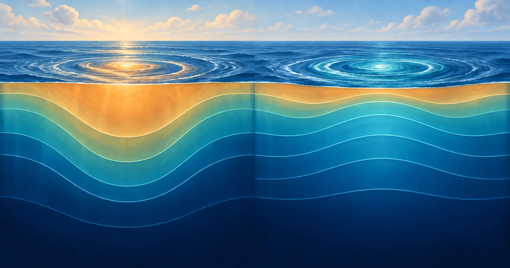
An isopycnal connects water with the same density; when comparing vertically separated water, oceanographers commonly use a potential-density surface with a stated reference pressure to account for compression. In a typical surface-intensified anticyclone, these surfaces are depressed toward the center. In a corresponding cyclone, they dome upward. A global analysis by Chen and colleagues (2021) documents the associated deepening and lifting of the pycnocline.
Where temperature decreases downward and salinity differences do not reverse the density pattern, a downward displacement extends warmer water to greater depth. An upward displacement puts colder water at the same comparison depth. The general layer structure is introduced in How Does the Ocean Change With Depth?.
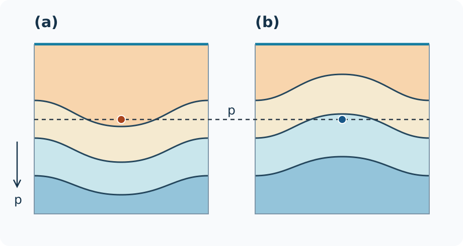
(a) A warm-core eddy; (b) a cold-core eddy. Solid curves show surfaces of equal potential density; the dashed line marks a common pressure, p.
A depressed layer is not evidence that water is continually sinking there. Its shape records the structure at the observation time; determining ongoing upwelling or downwelling requires information about how the flow and layers evolve.
Why salinity matters
There is no universal rule that a warm eddy is salty and a cold eddy is fresh. Salt can reinforce or offset temperature’s influence on density. The Japan Meteorological Agency documents cold, fresh anticyclonic eddies associated with water originating in the Sea of Okhotsk: their low salinity contributes to low density despite their low temperature. This is a concrete exception to inferring rotation from temperature alone. See JMA’s warm- and cold-eddy explanation.
Are the Layers Moving, or Are the Water Properties Different?
Suppose a thermocline is deeper in one profile than in a nearby reference profile. A warmer value at 200 dbar could result from that displacement even if the temperature-salinity relationship of the water is unchanged. This idealized vertical rearrangement is called heave.
Two comparisons help separate the possibilities:
- At the same pressure: compare temperature and salinity where both profiles have valid data. This shows the difference experienced at a particular level.
- On the same potential-density surface: compare the pressure where that surface occurs, then the temperature and salinity on it. A pressure shift with similar water properties is consistent with heave. A remaining temperature-salinity difference indicates a property contrast that pure heave cannot explain.
The second comparison requires an explicit density calculation and an appropriate reference pressure. For an upper-ocean comparison using σ₀, the TEOS-10 definition of σ₀ uses Absolute Salinity and Conservative Temperature. Do not feed potential temperature directly into a function that expects Conservative Temperature.
A θ-S diagram helps compare the relationships, but similar curves do not prove that the profiles sampled the same water mass or its motion. Their depth information must be checked separately. Conversely, warmer and saltier water can have similar potential density to colder, fresher water. Water Masses, Temperature, Salinity, and T-S Diagrams explains why assigning an origin requires more evidence.
A Published Argo Comparison: Different Core Depths off Peru and Chile
Chaigneau and colleagues (2011) combined Argo profiles with satellite altimetry in the eastern South Pacific. Their composite cyclonic core was centered near 150 m, while the anticyclonic core was near 400 m. Temperature and salinity departures from the study’s background were negative in the cyclonic core and positive in the anticyclonic core.
These are averages assembled from many profiles and eddies. In this region, the largest subsurface temperature and salinity differences occur at different depths for the two eddy types, beyond what surface maps reveal.
Subsurface-intensified anticyclones can also have a lens-like structure: density surfaces rise above the core and sink below it. Such structures, described by Zhang and colleagues (2017), do not fit a picture in which all the layers simply bend downward. Their surface expression can be weak.
Plan an Argo Comparison Around an Eddy
An eddy interpretation needs evidence for the circulation as well as the water properties. Use a regional study or a contemporaneous external sea-surface-height or velocity analysis to establish the candidate eddy’s position and extent. Check the date and the method used to define it.
Within that context, compare profiles near the estimated center, nearer the edge, and outside the feature. Keep dates close and the surrounding reference on the same side of any large front when possible; otherwise, a background regional gradient may dominate the difference. Ocean Fronts and Temperature-Salinity Profiles explains that additional complication.
Check each profile’s UTC date, position, WMO ID, and cycle number. At common pressure levels, compare the thermocline position, salinity extrema, and the depth range over which differences persist. Keep missing values as gaps and check the original Argo QC flags before treating an isolated feature as physical.
A standard Argo cycle is about 10 days, with much of that time spent drifting near 1,000 m before profiling upward from around 2,000 m; individual missions differ. The International Argo Program’s float-cycle description explains the sequence. The float and eddy can both move between profiles, so a sequence mixes spatial and temporal change. It may miss the center entirely. A loop in the float’s surface positions is also insufficient to establish the eddy’s surface circulation or speed.
What You Can Check in OceanGraph
OceanGraph supports the initial profile comparison.
- Search a focused area and period. Use the external eddy reference to choose the map area. The Search and Bookmark guide describes geographic and UTC date filters.
- Inspect potential temperature and Absolute Salinity. Select map markers one at a time and inspect the profiles alongside their dates and positions. For an overlay, download the selected profile JSON files and upload them to the desktop Analysis Lab: Vertical Profiles viewer.
- Compare θ-S structure. Selecting a marker highlights that profile’s curve. The background σ₀ contours provide density context. With Trajectory off, Analyze → Generate θ-S uses the entire current search result, limited to 500 profiles.
- Examine repeated profiles with their positions. A time-series vertical section can reveal changes in layer depth; return to each cycle’s date and location before interpreting them as eddy evolution. Trajectory loads all available cycles for the chosen float, including cycles outside the original date filter.
The θ-S Diagram guide and Trajectory and Time-Series Vertical Section guide explain the displays. OceanGraph’s downloaded JSON contains processed profile values rather than the source QC arrays; consult the Data Filtering Policy and obtain the corresponding original Argo NetCDF when checking data quality.
For the forces behind the circulation, continue with What Causes Ocean Currents?. If the main difference is a changed temperature-salinity relationship, the next step is to examine water-mass properties and their interpretation.