Reading Argo Data in Python: What to Decide Before You Write Code

Loading Argo data into Python is a few lines. Loading the right Argo data is a set of decisions that the few lines quietly make on your behalf — which files to read, whether to use raw or adjusted values, which quality flags to accept, and what the vertical coordinate means.

Getting those wrong does not usually raise an error. It produces plausible numbers that are subtly not what you meant. This guide covers the choices, shows what each one does to a real float’s data, and points out the places where the first attempt tends to break.

If you have not opened an Argo file at all yet, Argo NetCDF Format Explained for Beginners covers the structure this guide assumes.

Two Routes, Different Amounts of Responsibility

There are two realistic ways to get Argo profiles into Python.

argopy is a library maintained by the Euro-Argo development community that handles discovery, download, caching, and quality filtering, and returns an xarray Dataset. xarray with netCDF4 reads GDAC files directly and hands you exactly what is in them.

	argopy	xarray + raw NetCDF
Finding files	Query by region, float, or profile	You locate them yourself
QC and data mode	Applied for you, per user mode	Yours to apply
Output shape	Tidy Dataset, reshapeable	The file’s own dimensions
Unfiltered data	Available via expert mode	Always

The choice is not about skill level. argopy is the better default for almost any analysis that starts from a question about a region or a float. Raw NetCDF is the right route when you need something argopy does not expose, when you are working from a local mirror, or when you need to know exactly what the file said before anything touched it.

argopy in Three Lines

from argopy import DataFetcher

ds = DataFetcher(src="erddap", mode="standard").float(6902746).load().data

That returns an xarray Dataset in a “point” layout: every measurement at every level of every cycle is one row along an N_POINTS dimension, with LATITUDE, LONGITUDE, and TIME as coordinates. It is a convenient shape for filtering and awkward for plotting a profile, so argopy provides a reshape:

profiles = ds.argo.point2profile()

which gives the familiar N_PROF × N_LEVELS layout.

Two arguments in that first line matter more than the rest.

src selects where the data comes from: erddap (the default), gdac (the official servers, or a local GDAC-compliant directory), or argovis. Biogeochemical parameters come from erddap or gdac; argovis serves core data only. mode selects how much processing argopy applies before you see anything.

The User Mode Is a Scientific Decision

argopy has three user modes, and they are not verbosity settings. They change which measurements exist in your Dataset.

• expert returns the data as the source holds it, with no filtering. Raw and adjusted variables both present, all quality flags included.
• standard (the default) keeps measurements whose quality flags are 1 or 2, merges PARAM_ADJUSTED into PARAM and drops the separate adjusted variables, and hides variables that only experts need.
• research is stricter again: delayed-mode data only, quality flag 1 only, and a pressure error limit on core parameters.

For one float — WMO 6902746, a delayed-mode float with 138 cycles — the three modes return:

Mode	Measurements	Profiles	Variables
expert	14,345	138	23
standard	12,518	118	15
research	12,518	118	9

Expert mode matches the float’s multi-profile file at the GDAC exactly, which is a useful confirmation that the source is faithful. Standard mode then removes about thirteen percent of the measurements and twenty whole profiles. Those are not errors in argopy — they are quality decisions the Argo programme already made, applied for you.

The consequence is that a profile count from a script is a statement about your filtering as much as about the float. Record the mode alongside the result.

For what the flags and data modes mean before argopy applies them, Argo Data Quality Control is the reference.

The Raw NetCDF Route

Reading a GDAC file directly is one line:

import xarray as xr

ds = xr.open_dataset("6902746_prof.nc")

What you get back is the file’s own structure — for this float, N_PROF 138, N_LEVELS 110, plus N_PARAM, N_CALIB, and N_HISTORY. Nothing has been filtered, TEMP and TEMP_ADJUSTED both exist, and choosing between them is now your job.

The measurement arrays are rectangular, but the profiles are not. Every profile is padded out to the length of the longest one in the file, so a short profile is followed by missing values that carry no meaning.

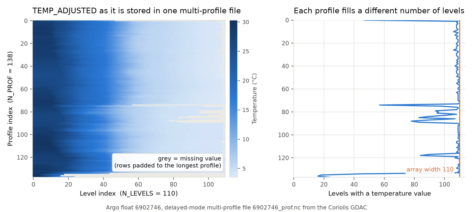
Most profiles in this file fill more than a hundred levels; a handful fill far fewer, one as few as 16. About five percent of the array is padding. Any statistic you compute across the level axis without masking those cells is averaging the padding into the answer.

Four Details That Break the First Attempt

The first three belong to the raw NetCDF route: argopy casts the flag and data-mode fields for you, and outside expert mode it resolves the raw-versus-adjusted choice as well. The last one applies whichever route you take.

Quality flags are bytes, not integers

QC variables are stored as single characters, so xarray hands you an object array containing byte strings, with floating-point NaN where a value is absent. Comparing that array to the integer 1 does not work, and sorting it raises a TypeError because it cannot order bytes against floats. Compare against byte literals instead:

import numpy as np

good = np.isin(ds["TEMP_QC"].values, [b"1", b"2"])

DATA_MODE has the same shape of problem: its values are b"R", b"A", or b"D", not the strings you might expect.

Pressure is not depth

Argo’s vertical coordinate is pressure in decibars, and the numeric closeness to metres is a rough guide rather than an identity: one decibar is near one metre of seawater because of the density of seawater and the strength of gravity, and neither is constant. Converting properly needs latitude, because gravity varies with it:

import gsw

depth_m = -gsw.z_from_p(2000.0, 30.0)

At 2,000 dbar that gives about 1,977 m at 30° latitude, against roughly 1,980 m at the equator and 1,972 m at 60°. Under one percent, but systematic, and the latitude dependence means the offset differs between the profiles you are comparing. For a threshold calculation, staying in decibars avoids the issue entirely.

Raw and adjusted must not be mixed

TEMP with TEMP_ADJUSTED_QC, or an adjusted temperature with a raw salinity, produces a profile that is not any measurement anybody made. Read the data mode first, select the matching value and flag fields, and keep the pairing consistent for every parameter. For biogeochemical parameters, the mode is per parameter — PARAMETER_DATA_MODE, not DATA_MODE.

Units are in the attributes, and they are not all what you expect

PRES carries decibar, TEMP carries degree_Celsius, and PSAL carries psu — practical salinity, not Absolute Salinity. Deriving density or Conservative Temperature means a TEOS-10 conversion first. Dissolved oxygen arrives as DOXY in µmol/kg, already converted from whatever the sensor reported; Dissolved Oxygen Units in Ocean Data covers why that matters when you combine it with another dataset.

Pin the Environment Before It Pins You

Argo tooling sits on a deep scientific Python stack, and the version combinations that work are not always the newest of everything. An analysis that runs today and fails in six months on a rebuilt environment is a common and avoidable outcome.

Recording exact versions — a lockfile, an environment file, or a container image — turns “it worked on my machine” into something a reviewer or a future you can reproduce. How to Make a Research Analysis Reproducible with Docker covers doing that without much ceremony.

Looking First Makes the Code Shorter

Most of the code people write against Argo in the first week is not analysis. It is finding out what the data looks like: which floats are in the region, whether a float’s cycles span the period, whether oxygen is present, whether the feature they are after is there at all.

That is a reading problem, and reading it visually is faster than writing a loader to answer it. Once you know which WMO IDs and cycles matter, argopy’s .float() and .profile() queries go straight to them, and the script you write is the analysis rather than the search.

Visualizing Argo Float Data Without Python covers that screening step in OceanGraph, and the App Guide documents Search and Bookmark. None of it removes the need for Python; it removes the need to write Python before you have a question worth writing it for.

Frequently Asked Questions

Should I use argopy or read NetCDF files directly?

Use argopy unless you have a reason not to. It handles discovery, caching, and the quality decisions consistently, and its expert mode gives you the unfiltered data when you need it. Read files directly when you are working from a local mirror, need a variable argopy does not expose, or want to verify exactly what the file contains.

Why does my profile count change when I change the mode?

Because the modes apply different quality-control and data-mode filters. Standard mode keeps flags 1 and 2; research mode keeps only delayed-mode data with flag 1. A profile with no surviving measurements disappears from the result entirely.

How do I filter by quality flag myself?

It depends on the route. Reading a file directly, compare against byte literals such as b"1" and b"2", since the flags are stored as characters rather than numbers. argopy casts its QC variables to integers, so filtering an expert-mode Dataset is ds.argo.filter_qc(QC_list=[1, 2]) on the accessor.

Can I convert pressure to depth without gsw?

You can approximate it, but a latitude-aware conversion is a single call in gsw and removes an avoidable source of error. If the analysis does not require metres, staying in decibars is simpler and matches how Argo reports the data.

Do I need Python at all for a first look?

No, and it is often faster not to. Screening profiles visually before writing code narrows what the code has to do. Python becomes necessary as soon as you need repeatable processing, custom derived quantities, or more profiles than you would open by hand.