
On this page
If you have downloaded Argo data and opened your first .nc file, the experience is often confusing. You expected ocean profiles. Instead, you got a long list of variables, dimensions, metadata fields, and quality-control flags.
That is why so many beginners search for an explanation of the Argo NetCDF format. The challenge is usually not whether the data exists. It is understanding how the file is organized and which parts matter first.
This guide explains what NetCDF is, how Argo profile files are typically structured, which variables you should inspect first, what beginners often misunderstand, and how to use OceanGraph to understand the data before building a full coding workflow.
If you want a profile-centered overview before the file-format details, start with How to Read Argo Float Data for Beginners (What to Look at First).
What Is NetCDF?
NetCDF stands for Network Common Data Form. It is a file format widely used for scientific data, especially when the data includes multiple variables, metadata, and dimensions such as time, depth, latitude, and longitude.
NetCDF is common in oceanography because it can store:
- Measurement arrays
- Coordinates
- Units
- Metadata
- Quality information
- Multiple dimensions in one file
That makes it powerful, but not always beginner-friendly.
When you open a NetCDF file, you do not see a narrative explanation of the observation. You see a data structure. Your first task is to translate that structure into a scientific question.
Why Argo Uses NetCDF
Argo data is more than a single column of temperature values.
A profile can include:
- Float identity
- Cycle information
- Position
- Time
- Pressure levels
- Temperature and salinity
- Quality flags
- Additional variables such as oxygen in some cases
NetCDF is useful because it keeps those components together in a consistent machine-readable format.
The downside is that the file is optimized for storage and exchange, not for beginner interpretation.
How to Think About an Argo File
The best way to understand an Argo NetCDF file is not to memorize every variable name. It is to think in layers.
At a high level, one Argo profile file usually combines:
- Observation context
- Measurement arrays
- Quality and status information
- Metadata about the platform or processing
If you read the file in that order, it becomes easier.
1. Observation Context: What Profile Am I Looking At?
Before worrying about the measurement arrays, identify the observation itself.
The first questions are:
- Which float produced this profile?
- Which cycle is it?
- When was it taken?
- Where was it reported?
Common fields you will often encounter include:
PLATFORM_NUMBERfor the float identityCYCLE_NUMBERfor the profile sequenceJULDfor time informationLATITUDELONGITUDE
The exact combination can vary depending on file type and processing level, but the goal stays the same: place the profile in time and space before interpreting the measurements.
This is important because Argo data is easiest to understand as an observation event, not as a list of variable names.
2. Measurement Arrays: What Was Observed Through the Water Column?
Once you know the profile context, move to the measurement arrays.
In many core Argo profile files, the most important variables are:
PRESTEMPPSAL
These usually represent:
- Pressure
- Temperature
- Practical salinity
Some files also include adjusted versions such as:
PRES_ADJUSTEDTEMP_ADJUSTEDPSAL_ADJUSTED
PRES, TEMP, and PSAL are the raw core variables: pressure, in-situ temperature, and Practical Salinity. Potential temperature and Absolute Salinity are derived quantities, not replacements for these standard variables in a core Argo profile file.
The practical beginner takeaway is simple:
- Start by identifying the main profile variables
- Check the data-mode field before choosing raw or adjusted values
- Do not try to interpret every variable at once
If you are using biogeochemical Argo data, you may also encounter variables such as dissolved oxygen or other sensor products. But for first-pass understanding, pressure, temperature, and salinity are usually enough.
3. Quality Information: Can I Trust Every Value Equally?
One reason Argo NetCDF files feel complicated is that they do not store measurements alone. They also store quality information.
You may see fields such as:
PRES_QCTEMP_QCPSAL_QCPOSITION_QC
The exact interpretation depends on the Argo conventions for the file, but the general point is consistent: not every value should be treated identically without checking its quality status.
For beginners, a useful rule is:
- Do not panic when you see QC fields
- Remember that quality information is part of responsible interpretation
- Select raw or adjusted values from the data mode, then use the matching QC and error fields before scientific interpretation
A questionable point or missing value does not automatically make the whole profile unusable.
4. Dimensions: Why Do the Arrays Have Different Shapes?
Another common point of confusion is the array structure.
Argo NetCDF files often organize values using dimensions such as:
- Number of profiles
- Number of vertical levels
- Number of parameters
That means some variables look like one-dimensional arrays, while others are stored across more than one dimension.
Beginners often get stuck here because they expect the file to behave like a simple spreadsheet. But the data is hierarchical:
- A profile file can contain one or more profile or sampling-scheme records
- A profile can have many depth or pressure levels
- Each level can have several measured variables
In version-3 profile files these are commonly represented by dimensions such as N_PROF, N_LEVELS, and N_PARAM. N_PROF can be greater than one when a cycle contains different vertical sampling schemes, so a cycle number is not always a one-to-one identifier for a single array of levels.
You do not need to master the full dimensional design immediately. What matters first is understanding which array corresponds to the water-column observations you want to inspect.
The First Variables to Check
If you open an Argo NetCDF file and want the fastest path to understanding, inspect the data in this order:
- Float identity
- Cycle number
- Time
- Latitude and longitude
DATA_MODE, orPARAMETER_DATA_MODEfor BGC parameters- Pressure, temperature, and salinity from the correct raw or adjusted fields
- Matching quality-control and error fields
This order matches the scientific workflow better than opening the file alphabetically.
It answers:
- What is this observation?
- Where and when did it happen?
- What does the water column look like?
- Are there any quality issues I need to keep in mind?
Raw vs Adjusted Variables
One detail that often confuses beginners is the presence of both raw-looking variables and adjusted variables.
You may see a pair such as:
TEMPTEMP_ADJUSTED
or
PSALPSAL_ADJUSTED
Adjusted values have had an Argo calibration or correction applied. That adjustment can be produced in real time (A) or during delayed-mode expert processing (D); it does not simply mean “a value corrected later.”
Use the data-mode fields rather than guessing from whether an adjusted array exists:
- In a core profile, read
DATA_MODE. ForR, usePARAMwithPARAM_QC. ForAorD, usePARAM_ADJUSTEDwithPARAM_ADJUSTED_QCand, when needed,PARAM_ADJUSTED_ERROR. - In a BGC profile,
DATA_MODEalone is not sufficient because each parameter can be processed differently. ReadPARAMETER_DATA_MODEfor each parameter and profile. ForAorD, use that parameter’s adjusted fields. ForR, only raw values exist, but Argo warns that raw BGC accuracy is generally unsuitable for direct scientific use by non-experts.
Do not combine a raw value with an adjusted QC flag, or mix raw and adjusted parameters without an explicit scientific reason.
Common Beginner Mistakes
Most problems come from reading the file in the wrong order.
Starting with file structure instead of observation context
If you begin with obscure variables and dimensions, the file feels abstract. Start with float, cycle, time, and location.
Treating one profile as the whole float
An Argo float produces many cycles. A single profile is one observation in a sequence, not the whole story.
Ignoring quality fields completely
You do not need to memorize every flag immediately, but you should apply the relevant data-mode and QC decisions before treating a value as scientifically usable. Visual plausibility is not a substitute for Argo QC.
Assuming pressure is just a cosmetic coordinate
Pressure is the core vertical coordinate in the profile and determines how you read the water-column structure.
Trying to understand everything before visualizing anything
This is one of the biggest workflow mistakes. A profile often becomes clearer once you see it plotted.
Example: A Better Way to Read an Argo NetCDF File
Suppose you open a profile file and see dozens of variable names.
A better beginner workflow is:
- Identify the float and cycle.
- Check the date and location.
- Find the pressure, temperature, and salinity arrays.
- Read the relevant data-mode field and select raw or adjusted variables accordingly.
- Apply the matching QC fields and inspect error estimates when the analysis requires them.
- Plot or inspect the selected, quality-controlled profile visually.
This sequence turns a confusing NetCDF file into a readable ocean observation.
The Traditional Workflow: Python First
Many people approach Argo NetCDF files by opening them directly in Python with a scientific library and then building plots from scratch.
That is a valid workflow, but beginners often hit several friction points:
- NetCDF feels unfamiliar
- Variable names are not self-explanatory at first
- Quality fields interrupt the first reading
- You may debug indexing before you understand the water column
- Comparing several files still takes setup
If your first goal is understanding rather than automation, this can be heavier than necessary.
If you plan to serve these profiles from your own web application, you also need to decide what happens before delivery and what happens in the browser. From NetCDF to the Browser: Designing a Web App for Ocean Data describes that division of work.
A Better First Step: Understand the Observation Before the File
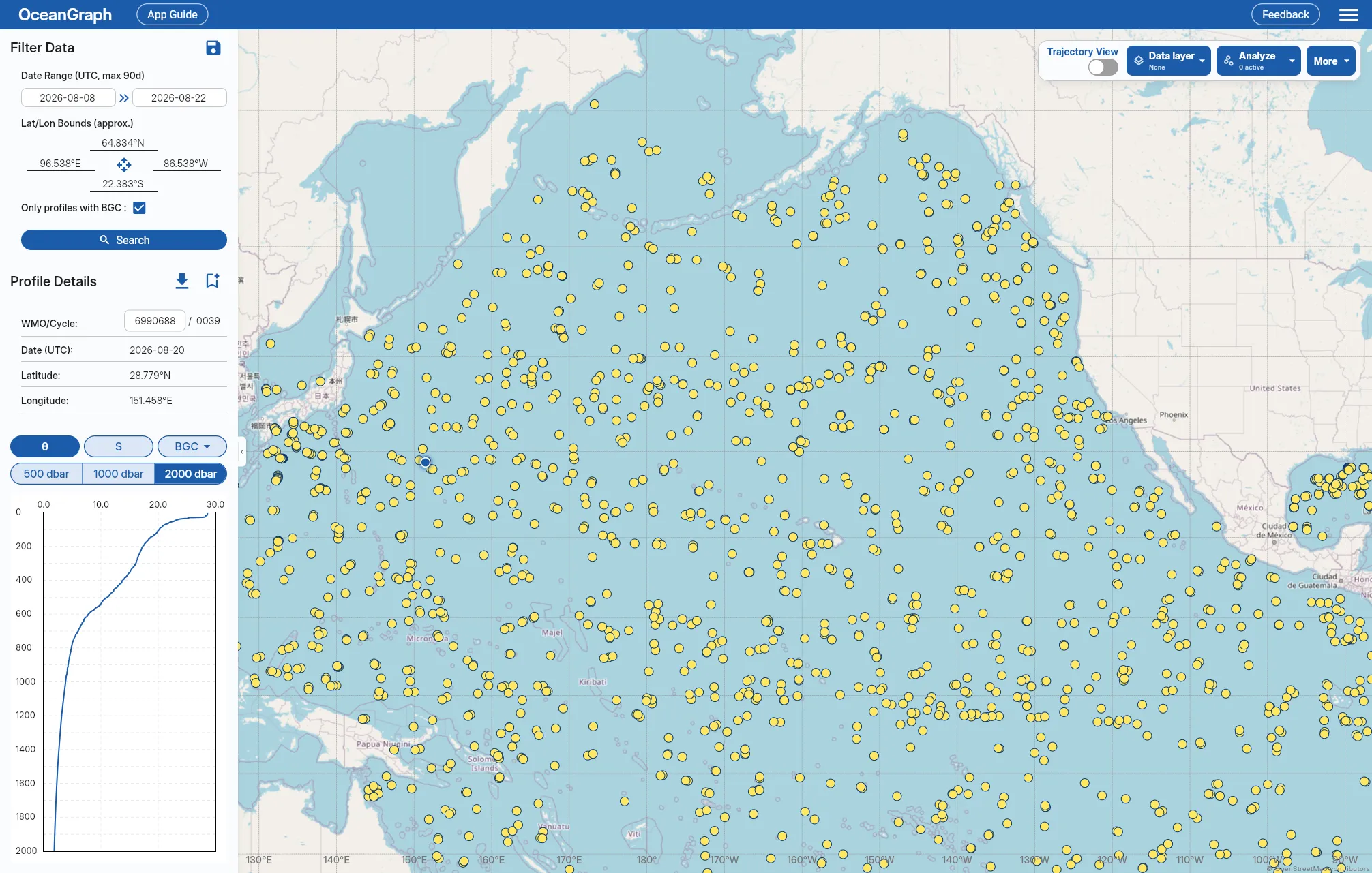
OceanGraph is useful because it lets you approach Argo data from the observation side first.
Instead of beginning with file parsing, you can:
- Search real profiles by region, time, and WMO ID
- Inspect the profile context directly
- Open vertical profiles immediately
- Compare several observations before deciding what to code later
Useful follow-up pages are:
- Search and Bookmark
- Analysis Lab: Vertical Profiles (JSON upload)
- Visualizing Argo Float Data Without Python (Step-by-Step Guide)
Once you already know which float, cycle, or pattern matters, the NetCDF file becomes much easier to approach.
Explore Argo Data Before You Parse the File
If you want to reduce file-format friction and understand what the data actually represents first, OceanGraph is a practical place to start.
OceanGraph helps bridge the gap between opening an Argo NetCDF file and understanding the ocean profile inside it.
Frequently Asked Questions
What does NetCDF mean in Argo data?
It refers to the scientific file format used to store Argo variables, coordinates, metadata, and quality information in a structured way.
What variables should I look at first in an Argo NetCDF file?
Start with float identity, cycle number, time, and location. Then read the relevant data mode, select the matching pressure, temperature, and salinity fields, and apply their QC and error information.
Why are there so many QC variables?
Because Argo data includes quality-control information alongside the measurements. That helps users interpret the data responsibly.
What is the difference between TEMP and TEMP_ADJUSTED?
TEMP is the raw in-situ temperature. TEMP_ADJUSTED is the calibrated or corrected value used when core DATA_MODE, or the BGC parameter’s PARAMETER_DATA_MODE, is A or D. Use the matching QC field for whichever value you select.
Do I need Python to start understanding Argo NetCDF files?
No. Python is useful for deeper analysis, but many beginners understand the data faster if they first inspect the observation visually and then return to the file structure.
Conclusion
The Argo NetCDF format feels difficult at first because it presents you with a data structure before it presents you with an observation. Once you read the file in a scientific order, the logic becomes much clearer: identify the profile, place it in time and space, select raw or adjusted values from the appropriate data mode, and apply the matching quality information before interpretation.
For many beginners, the fastest path is to look at real profiles first and approach the file only after the observation makes sense. That is where OceanGraph can help.
